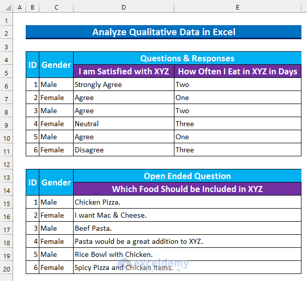
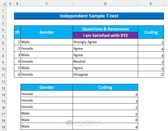
This dataset has 3 columns: “ID”, “Gender”, and “Questions & Responses”.
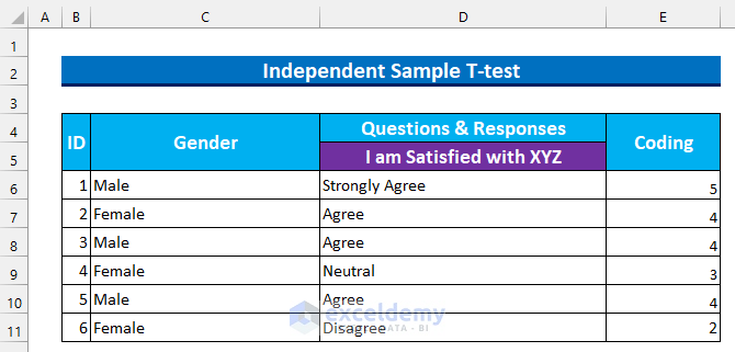
Step 1: Code and Sort Qualitative Data
Here, the Likert Scale has 5 levels:
- Strongly Agree -> 5.
- Agree -> 4.
- Neutral -> 3.
- Disagree -> 2.
- Strongly Disagree -> 1.
- Input values in the cell range E6:E11.
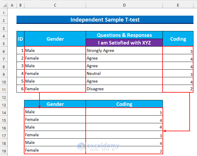
- Separate the “Gender” and “Coding” columns into different cell ranges.
- Select the cell range C14:D19 and right-click to see the Context Menu.
- From Sort >>> select “Sort A to Z”.
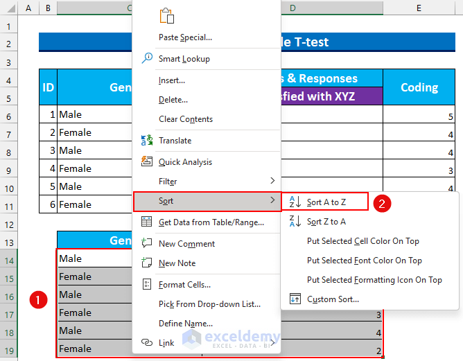
Values for the same gender will be displayed together.
Read More: How to Analyze Quantitative Data in Excel
Step 2: Enable the Analysis Toolpak
- Press ALT, F, then T to open Excel Options.
- From Add-ins >>> select “Go…”.
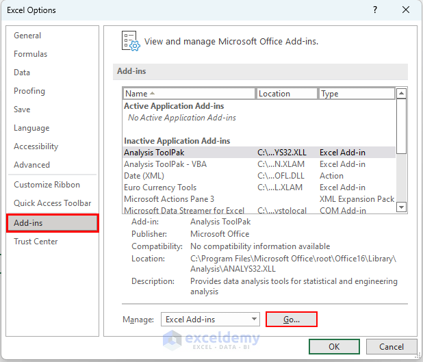
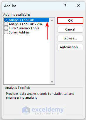
- In the Add-ins dialog box, select “Analysis Toolpak” and click OK.
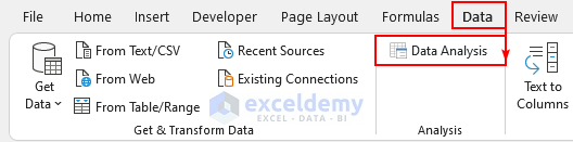
- Data Analysis will be displayed in the Data tab.
Read More: How to Analyse Qualitative Data from a Questionnaire in Excel
Step 3: T-test to Compare Means with Qualitative Data
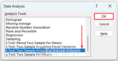
- In Analysis, click “Data Analysis”.
- Select “t-test: Two-Sample Assuming Unequal Variances” and click OK.
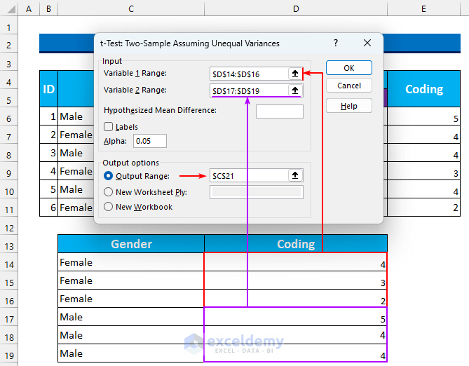
- In the dialog box , select:
- Variable 1 Range – D14:D16.
- Variable 2 Range – D17:D19.
- Select “Output Range” and C21 as the output location.
- Click OK.
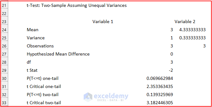
This will be the output.
The mean is 3 and 4.33. p-value will check whether this difference is significant. The variances are 1 and 0.33, so the assumption of unequal variances was correct. If this value is almost identical, change it to “t-test: Two-Sample Assuming Equal Variances”.
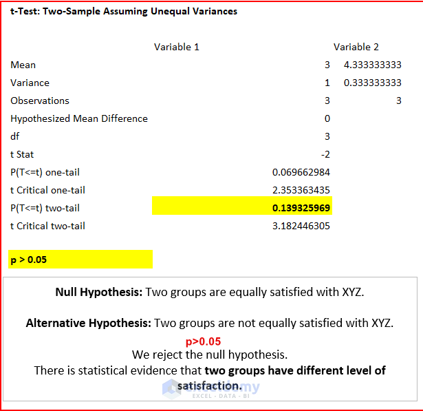
Focus on the P(T<=t) two-tail value only. It needs to be less than 0.05 to be significant. As it is 0.14 (more than 0.05), reject the null hypothesis.
The analysis shows that males and females have different levels of satisfaction with cafe XYZ, which is statistically significant.
Step 4: Prepare a Categorical Dataset for a Chi-Square Test
This is the sample dataset.
[/wpsm_box]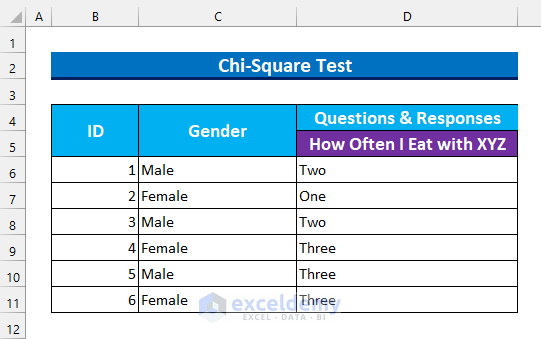
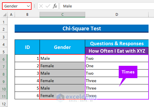
- Name the ranges C6:C11 as “Gender” and D6:D11 as “Times”.
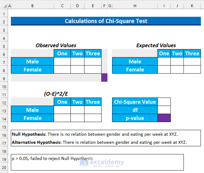
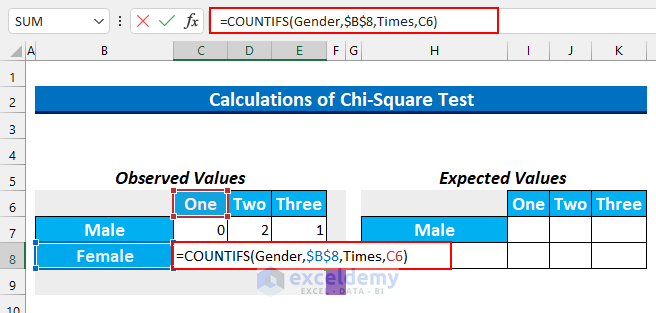
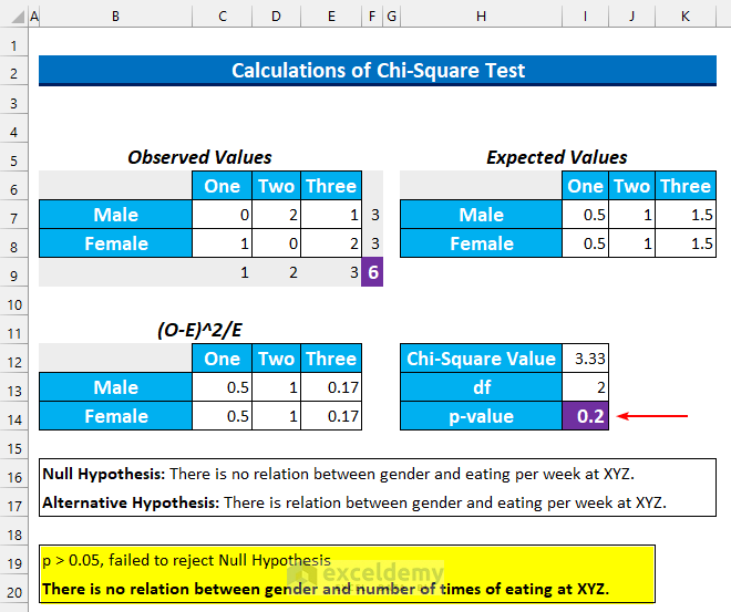
- Create a template to calculate the Chi-Squared value.
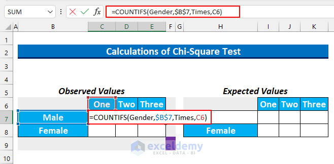
- Select C7:E7 and enter the following formula.
=COUNTIFS(Gender,$B$7,Times,C6)
This formula finds the number of cells with males and One time eating per week in cafe XYZ.
- Press CTRL+ENTER. This will AutoFill the formula.
- Select the cell range C8:E8 and enter the following formula.
=COUNTIFS(Gender,$B$8,Times,C6)
This formula finds the number of cells containing the females and eating once per week in the cafe XYZ.
- Press CTRL+ENTER.
- Sum the rows and columns.
- Select the cell range C9:E9 and enter this formula.
=SUM(C7:C8)
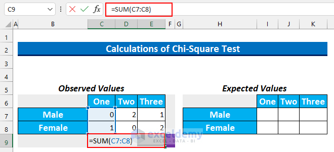
- Press CTRL+ENTER.
- Select the cell range F7:F8 and enter this formula.
=SUM(C7:E7)
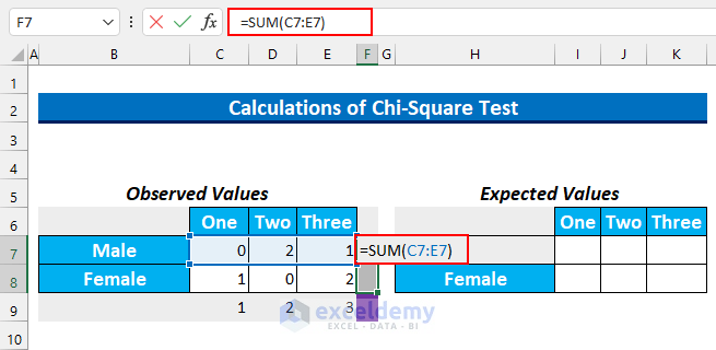
- Press CTRL+ENTER.
- Enter 6 in F9 (the number of respondents).
- To find the expected values, use the formula Row Total * Column Total/Total.
- Select the range I7:K and enter this formula.
=$F$7*C9/$F$9
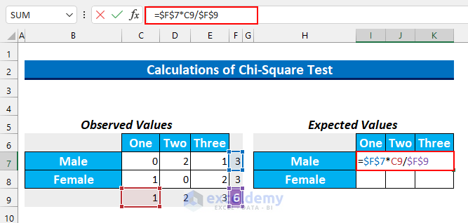
- Press CTRL+ENTER.
- Select the range I8:K8 and enter this formula.
=$F$8*C9/$F$9
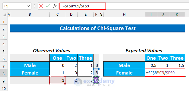
- Press CTRL+ENTER.
- Select the range C13:E14 and enter the following formula to find the Chi-Squared value.
=(C7-I7)^2/I7
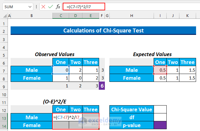
- Press CTRL+ENTER.
- Enter this formula to add these values in I12.
=SUM(C13:E14)
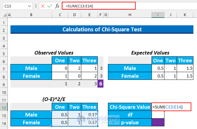
- Press ENTER.
df means degrees of freedom. The formula to find it is (Number of Columns -1) * (Number of Rows-1). There are 2 rows and 3 columns. Therefore, df is (3-1)*(2-1) = 2.
Read More: How to Convert Qualitative Data to Quantitative Data in Excel
Step 5: Analyze Categorical Qualitative Data with a Chi-Square Test in Excel
- Enter this formula in cell I14.
=CHISQ.DIST.RT(I12,I13)
This function returns “the right-tailed probability of the chi-squared distribution”.
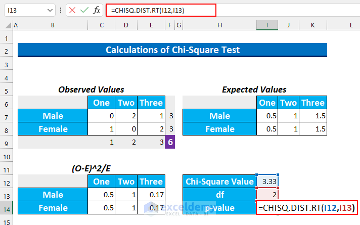
- Press ENTER.
The formula returns 0.2 which is bigger than 0.05. So, the reject the null hypothesis fails: the two categories have no relationship.
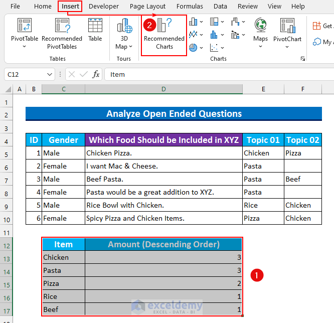
Step 6 – Sentiment Analysis for Open-Ended Qualitative Data
Two columns were added to the dataset: “Topic1” and “Topic2”.
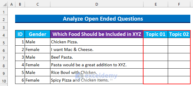
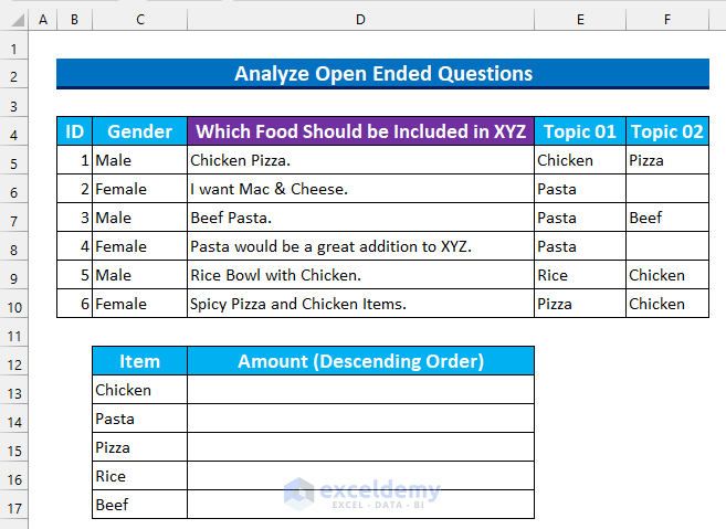
- You should read the responses and link them to food topics. For example, “Chicken Pizza” has 2 topics: “Chicken” and “Pizza”.
- Each topic is then added to a new table.
Step 7 – Use the COUNTIF Function to Analyze Open-Ended Qualitative Data
- Select D13:D17 and enter the following formula.
=COUNTIF($E$5:$F$10,C13)
This formula counts the number of values in F5:F10 that match the value in C13.
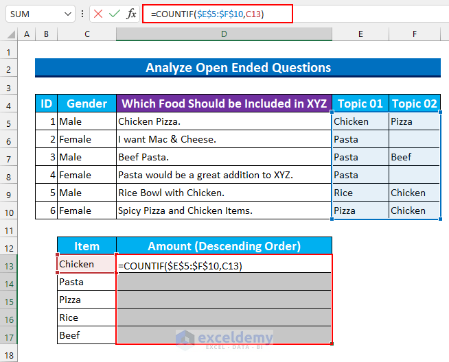
- Press CTRL+ENTER to AutoFill the formula.
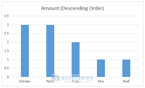
- Insert a Chart to see the frequency distribution.
Step 8 – Using a Clustered Column Chart to Visualize Open-Ended Qualitative Data
- Select C12:D17.
- From the Insert tab, select Recommended Charts.
- In the Insert Chart dialog box, select Clustered Column (it may be selected by default).
- Click OK.

The top 3 food items in the XYZ cafe are Chicken, Pasta, and Pizza.
Read More: How to Analyze Raw Data in Excel
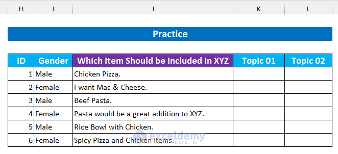
Practice Section
Practice with the following dataset.
Related Articles
- How to Analyze Large Data Sets in Excel
- How to Analyze Text Data in Excel
- How to Analyze Time Series Data in Excel
- How to Analyze Sales Data in Excel
- How to Analyze Likert Scale Data in Excel
- How to Analyze qPCR Data in Excel
<< Go Back to Data Analysis with Excel | Learn Excel
Get FREE Advanced Excel Exercises with Solutions!
