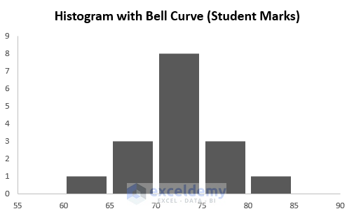
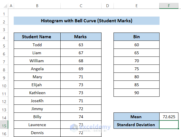
Method 1 – Histogram with Bell Curve for Student Marks
Steps
- Enable the Data Analysis Tool.
- Go to the File tab in the ribbon.
- Select the More command.
- In the More command, select Options.
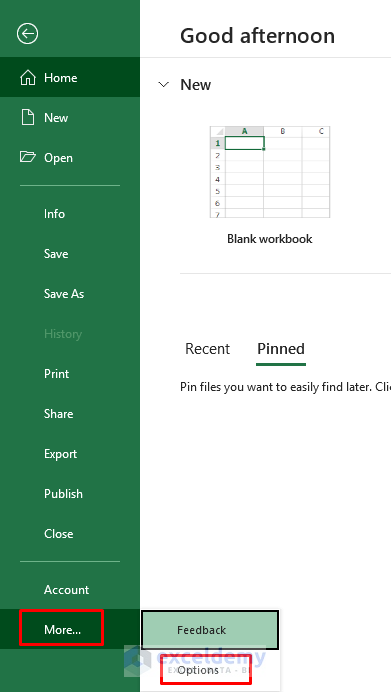
- An Excel Options dialog box will appear.
- Click on Add-ins.
- Click on Go.
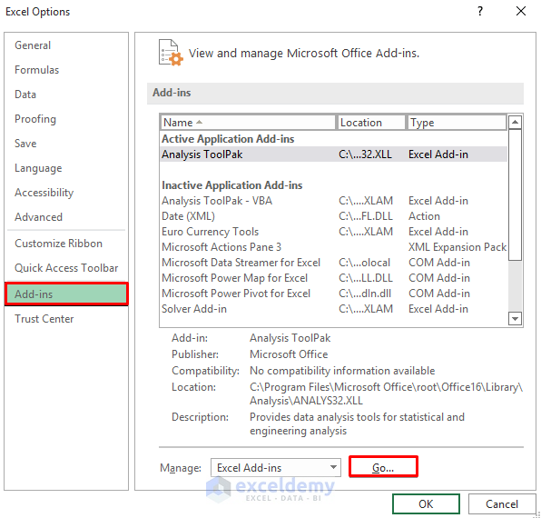
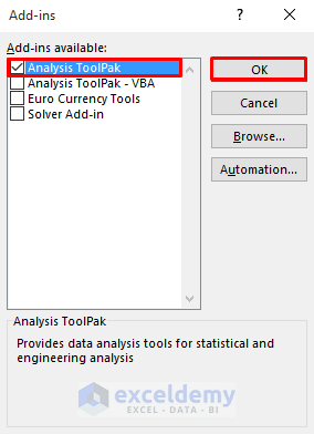
- From the Add-ins available section, select Analysis Toolpak.
- Click OK.
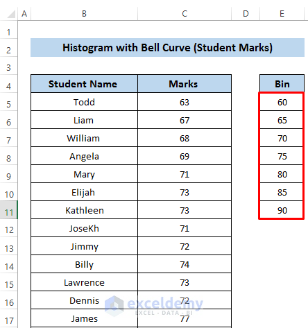
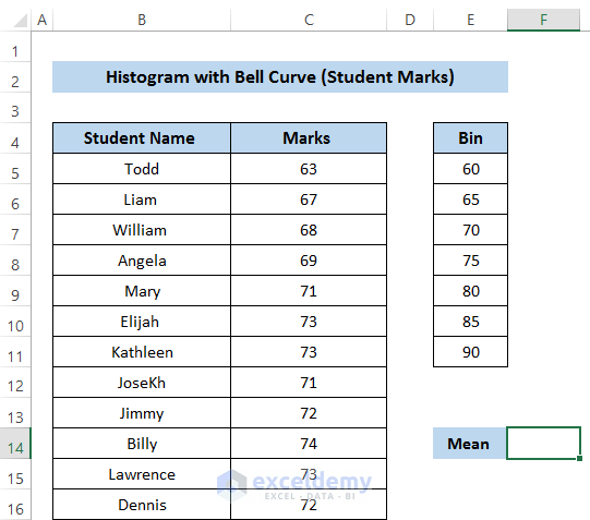
- To use the Data Analysis Tool, you need to have a Bin range.
- We set a bin range by studying our dataset’s lowest and highest values.
- We take intervals of 5.
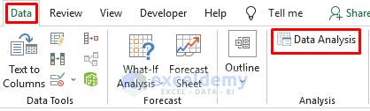
- Go to the Data tab in the ribbon.
- Select Data Analysis from the Analysis group.
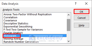
- A Data Analysis dialog box will appear.
- From the Analysis Tools section, select Histogram.
- Click OK.
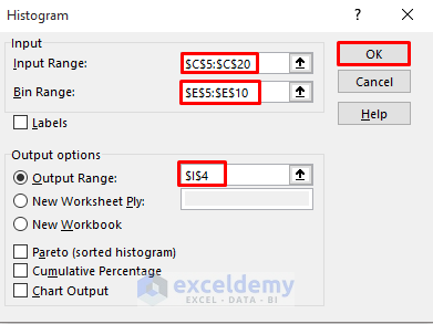
- In the Histogram dialog box, select the Input Range.
- Take the Marks column as the Input Range from cell C5 to cell C20.
- Select the Bin Range that we created above.
- Set the Output options in the current worksheet.
- Click on OK.
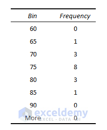
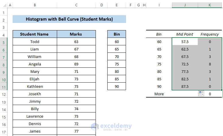
- It will give us the following output, which shows the bin we assigned previously and the frequency of distribution of our dataset. Bin 65 has 1 frequency, which means that from 60 to 65, they have found one mark of a particular student.
- To have a better chart, we need to add a new column and name it the midpoint of the bin instead of the endpoint of that bin.
- In the new column, write down the following formula.
=I5-2.5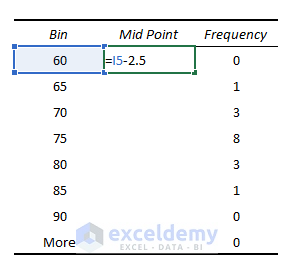
- Press Enter to apply the formula.
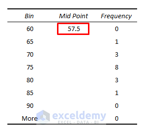
- Drag the Fill Handle icon down the column.
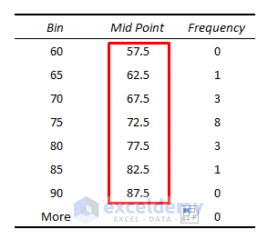
- Select the range of cells J5 to K11.
- Go to the Insert tab in the ribbon.
- From the Charts group, select Scatter Chart. See the screenshot.
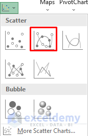
- From the Scatter chart, select the Scatter with Smooth Lines and Markers.
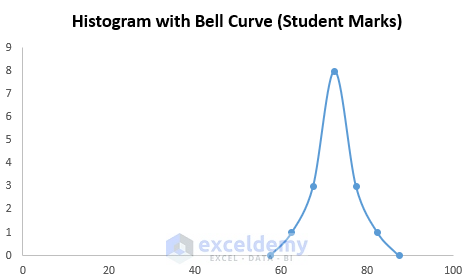
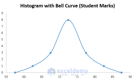
- It will give us the following chart using our dataset.
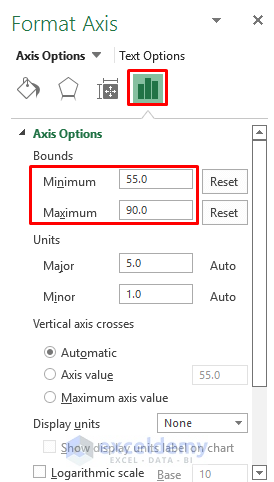
- To make the curve bigger and take it to the center, we need to adjust the x-axis.
- Double-click on the x-axis to open the Format Axis dialog box.
- After that, select the bar icon.
- Change the Minimum and Maximum values. This range is basically by studying the dataset.
- We get a bigger and center shape curve. See the screenshot.
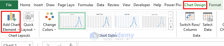
- You select the chart, a Chart Design will appear.
- Select the Chart Design.
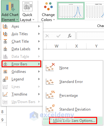
- From the Chart Layouts, select Add Chart Element.

- In the Add Chart Element option, select Error Bars.
- From the Error Bars, select More Error Bars Options.
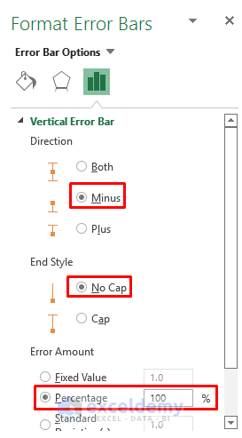
- A Format Error Bars dialog box will appear.
- In the Vertical Error Bar section, select direction Minus.
- Set End Style as No Cap.
- In the Error Amount section, set the Percentage to 100%.
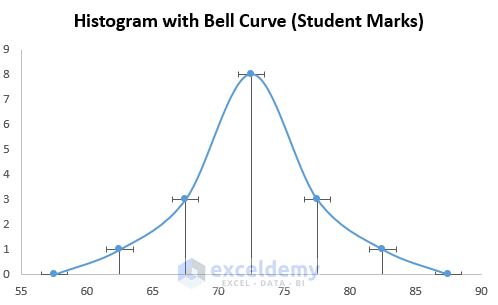
- It will represent the curve in the following way; see the screenshot.
- See the line in every bin, we need to change the line into a bar.
- Again go to the Format Error Bars.
- Change the Here, we take the width as 40.

- It will shape the curve in the following way. See the screenshot.
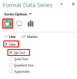
- Now we need to remove the curve because we have to draw the bell curve here.
- To delete the curve, click on the curve.
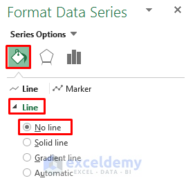
- A Format Data Series dialog box will appear.
- In the Line section, select No line.
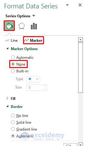
- Go to the Marker section.
- In the Marker options, select None.
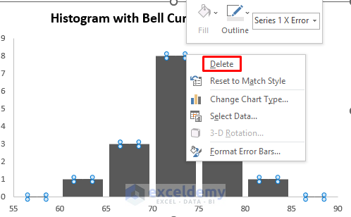
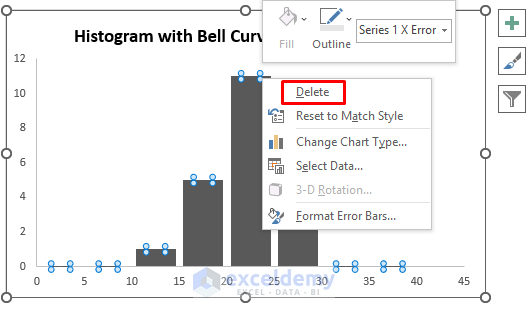
- All the lines and markers are gone. But there are some endpoints also in there.
- To remove them, click on them.
- Right-click to open the Context Menu.
- Select Delete to remove all the endpoints.
- We get the desired histogram from our dataset.
- We turn our focus to the bell curve.
- Before plotting the bell curve, we need to calculate the Mean, Standard Deviation, and the Normal Distribution.
- We need to find the Mean value of the student marks using the AVERAGE function.
- Select cell F14.
- Write the following formula in the formula box.
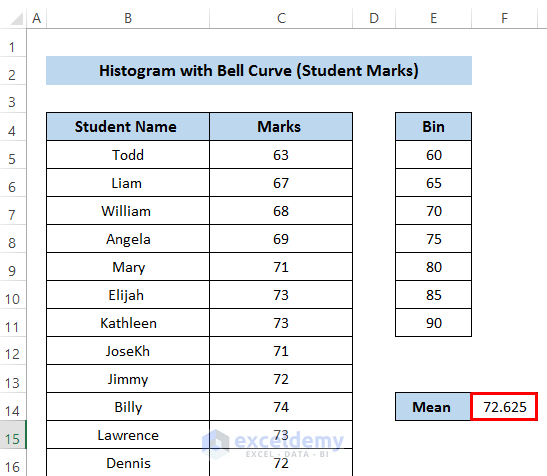
=AVERAGE(C5:C20)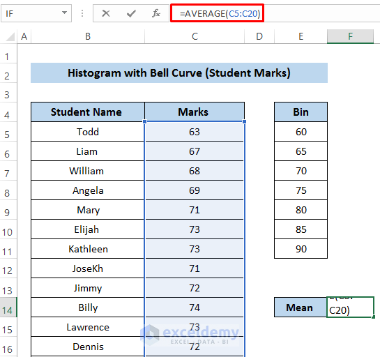
- Press Enter to apply the formula.
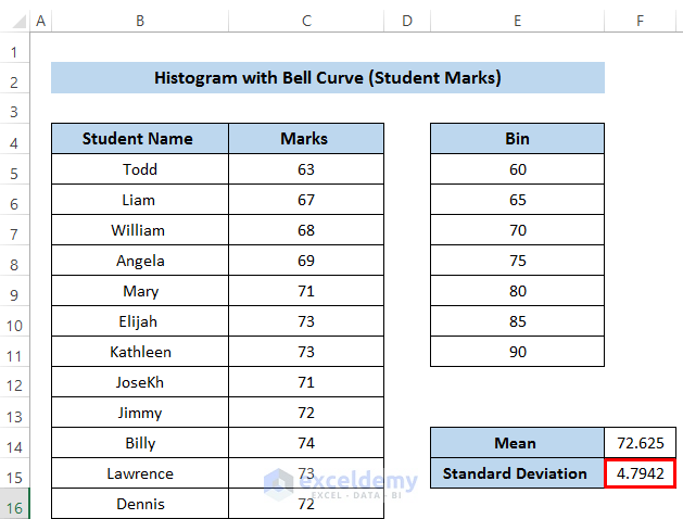
- We need to calculate the standard deviation using the STDEV.P function
- First, select cell F15.
- Write down the following formula in the formula box.
=STDEV.P(C5:C20)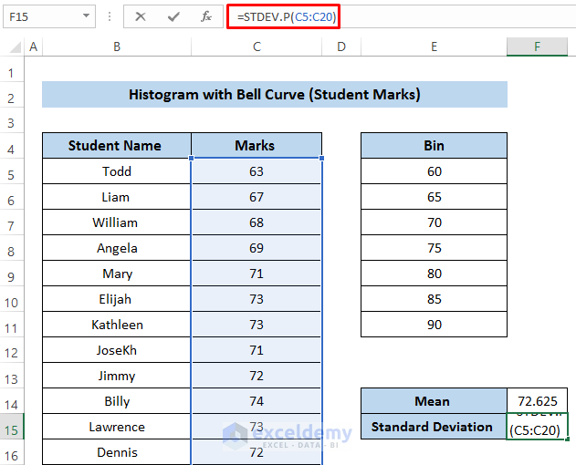
- Press Enter to apply the formula.
- Calculate the normal distribution to establish the bell curve.
- We take some values from 60 to 85. This value is taken by studying the histogram properly.
- Find the normal distribution for the corresponding values.
- Determine the regular distribution by using the NORM.DIST function.
- Select cell C26.
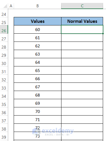
- Write down the following formula in the formula box. We need to scale the normal distribution in terms of the histogram graph. That’s why we use 97.
=NORM.DIST(B26,$F$14,$F$15,FALSE)*97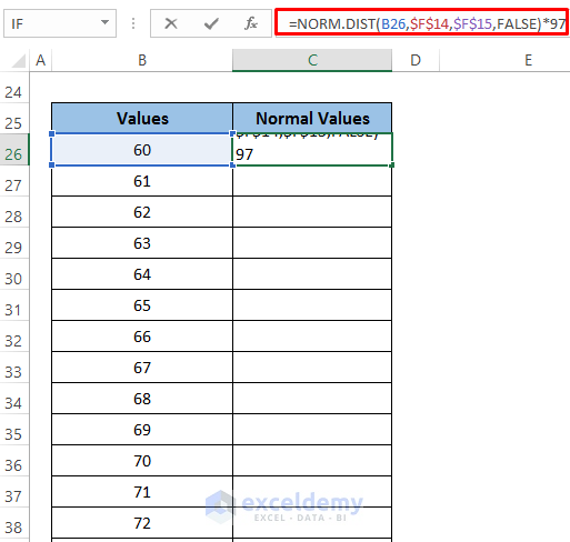
- Press Enter to apply the formula.
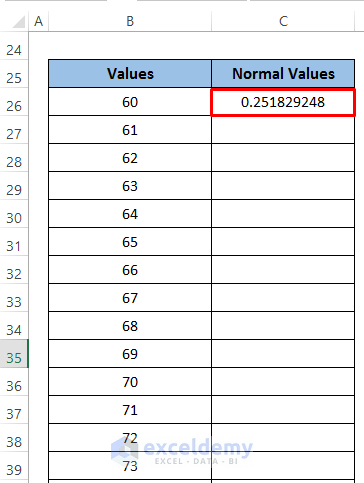
- Drag the Fill Handle icon down the column.
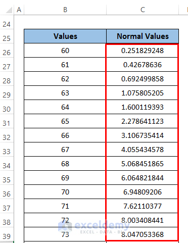
- Add the bell curve to the histogram curve.
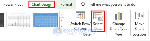
- Select the histogram chart that was made previously. It will open up the Chart Design option.
- From the Data group, click on Select Data.
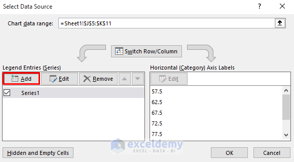
- A Select Data Source dialog box will appear.
- Select Add to insert new series.
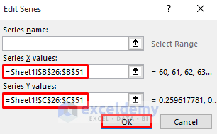
- In the Edit Series dialog box, select X and Y values range of cells.
- In the Y series, we set the normal distribution, in the X series, we set the values.
- Click OK.
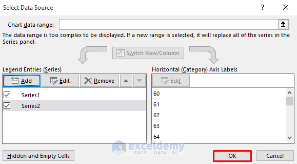
- Add as Series 2 in the Select Data Source dialog box.
- Click OK.
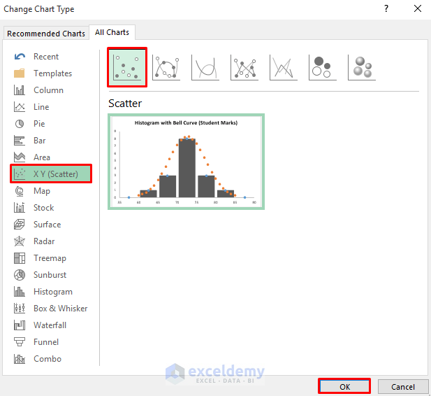
- Go to the Chart Design and Select Change Chart Type from the Type group.
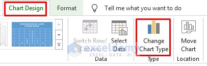
- Select the Scatter type chart. See the screenshot.
- Click OK.
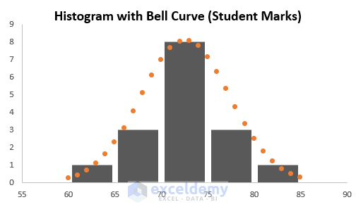
- It will give the bell curve along with the histogram. The curve line is in dotted format.
- We need to make it a solid line.
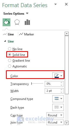
- Double-click the dotted curve, and the Format Data Series dialog box will appear.
- In the Line section, select Solid line.
- Change the Color.
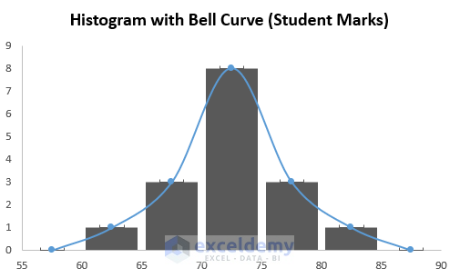
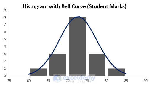
- We have our final histogram result with a bell curve for student marks.
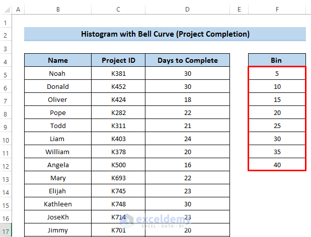
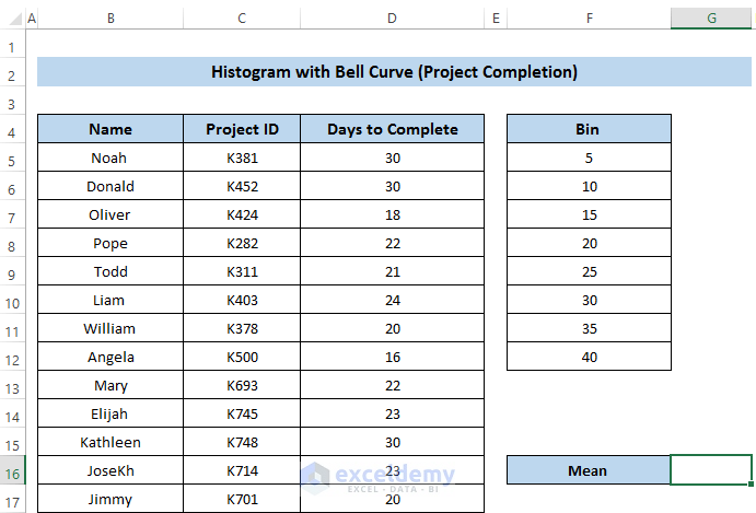
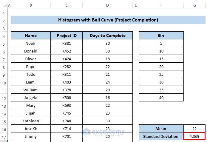
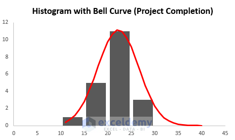
Method 2 – Histogram with Bell Curve for Project Completion
Steps
- To create a histogram, you need to use Data Analysis Tool.
- Use the Data Analysis Tool, you need to have a Bin range.
- We set a bin range by studying our dataset’s lowest and highest values.
- We take interval 5.
- Go to the Data tab in the ribbon.
- Select Data Analysis from the Analysis group.
- A Data Analysis dialog box will appear.
- From the Analysis Tools section, select Histogram.
- Click OK.
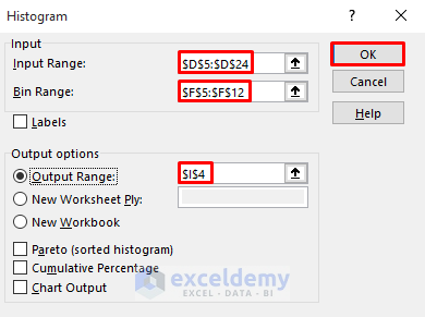
- In the Histogram dialog box, select the Input Range.
- Take the Marks column as the Input Range from cell D5 to cell D24.
- Select the Bin Range that we created above.
- Set the Output options in the current worksheet.
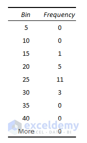
- Click OK.
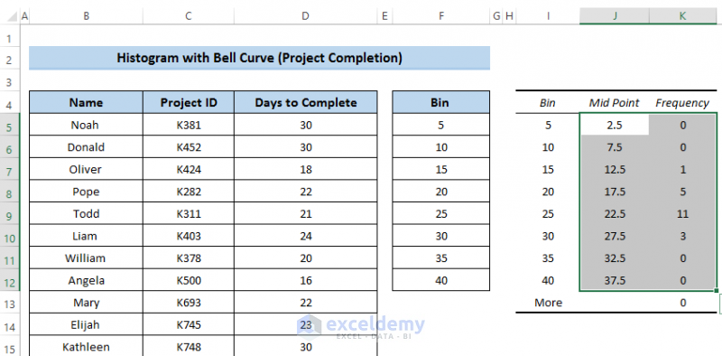
- It will give us the following output, which shows the bin we assigned previously and the frequency of distribution of our dataset. Bin 15 has 1 frequency, which means that from 10 to 15, they have found one mark of a particular student.
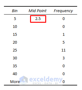
- Have a better chart, we need to add a new column and name it the midpoint of the bin instead of the endpoint of that bin.
- In the new column, write down the following formula.
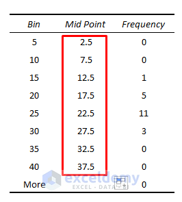
=I5-2.5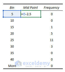
- Press Enter to apply the formula.
- Drag the Fill Handle icon down the column.
- Select the range of cells J5 to K12.
- Go to the Insert tab in the ribbon.
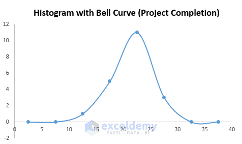
- From the Charts group, select Scatter Chart. See the screenshot.
- From the Scatter chart, select the Scatter with Smooth Lines and Markers.
- It will give us the following chart using our dataset.
- Select the chart, a Chart Design will appear.
- Select the Chart Design.
- From the Chart Layouts, select Add Chart Element.
- In the Add Chart Element option, select Error Bars.
- From the Error Bars, select More Error Bars Options.
- A Format Error Bars dialog box will appear.
- In the Vertical Error Bar section, select direction Minus.
- After that, set End Style as No Cap.
- In the Error Amount section, set the Percentage to 100%.
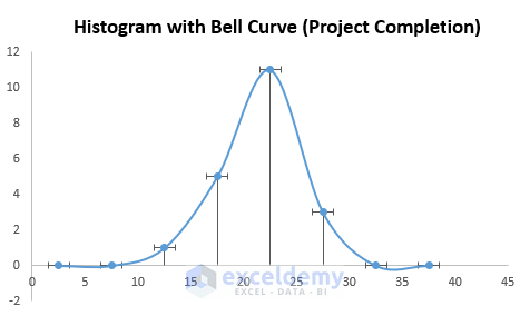
- It will represent the curve in the following way; see the screenshot.
- As you can see the line in every bin, we need to change the line into a bar.
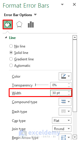
- Go to the Format Error Bars.
- Change the Here, we take the width as 30.
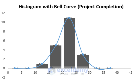
- It will shape the curve in the following way. See the screenshot.
- Now we need to remove the curve because we have to draw the bell curve here.
- To delete the curve, click on the curve.
- A Format Data Series dialog box will appear.
- In the Line section, select No line.
- Go to the Marker option.
- In the Marker options, select None.
- All the lines and markers are gone. But there are some endpoints also in there.
- To remove them, click on them.
- Right-click to open the Context Menu.
- Select Delete to remove all the endpoints.
- We get the desired histogram from our dataset.
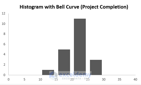
- We turn our focus to the bell curve.
- Before plotting the bell curve, we need to calculate the Mean, Standard Deviation, and the Normal Distribution.
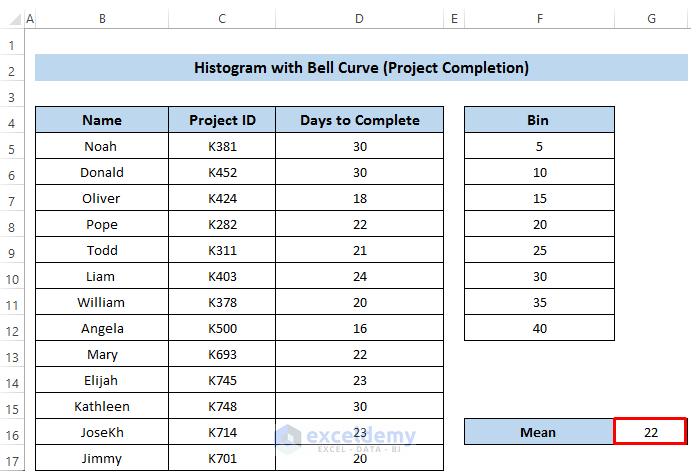
- We need to find the Mean value of the student marks using the AVERAGE function.
- Cell G16.
- Write the following formula in the formula box.
=AVERAGE(D5:D24)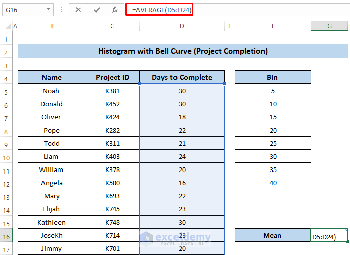
- Press Enter to apply the formula.
- Calculate the standard deviation using the STDEV.P function.
- Select cell G17.
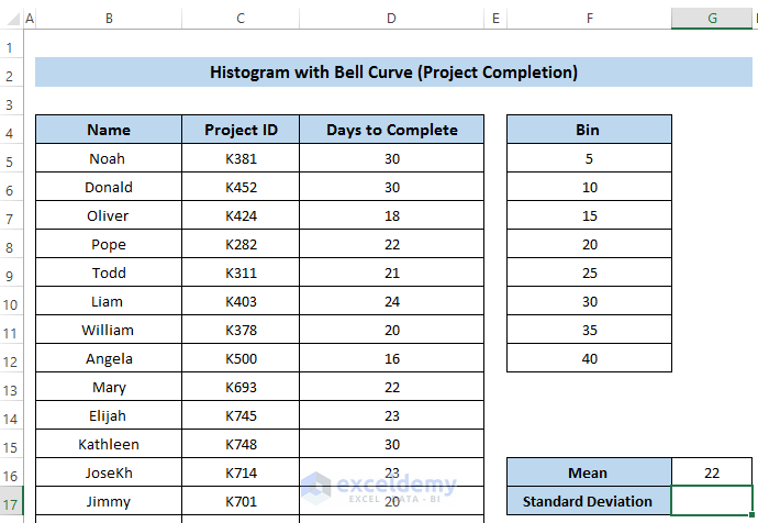
- Write down the following formula in the formula box.
=STDEV.P(D5:D24)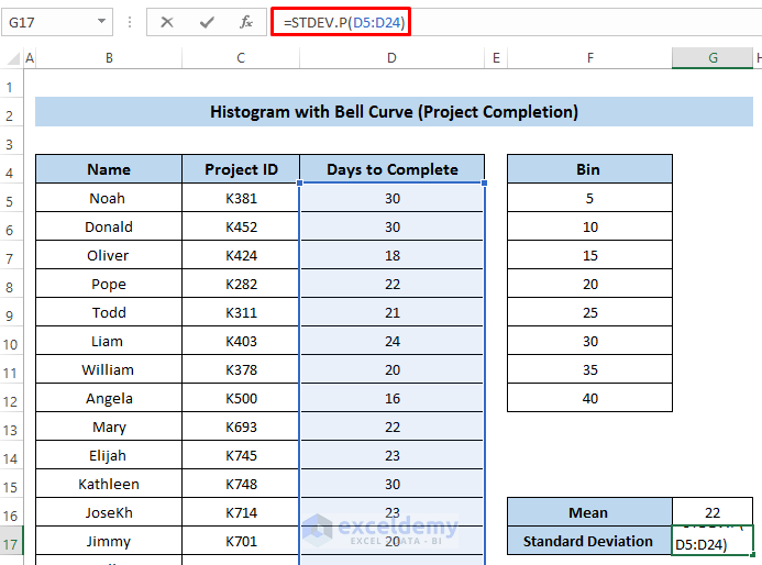
- Press Enter to apply the formula.
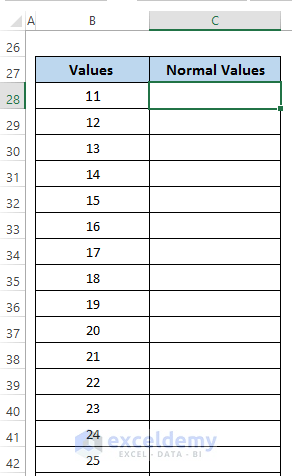
- Calculate the normal distribution to establish the bell curve.
- We take some values from 11 to 40. This value is taken by studying the histogram properly.
- Find the normal distribution for the corresponding values.
- Determine the regular distribution by using the NORM.DIST function.
- Select cell C28.
- Write down the following formula in the formula box. We need to scale the normal distribution in terms of the histogram graph. That’s why we use 122.
=NORM.DIST(B28,$G$16,$G$17,FALSE)*122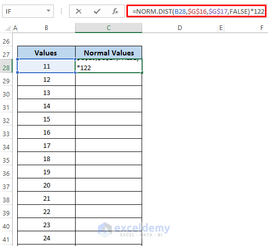
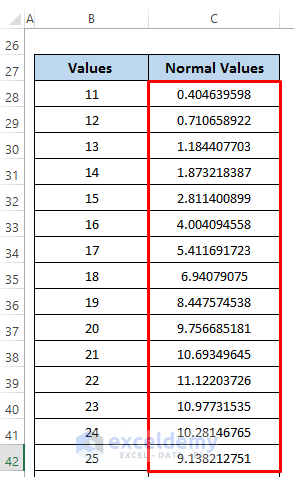
- Press Enter to apply the formula.

- Drag the Fill Handle icon down the column.
- Add the bell curve to the histogram curve.
- Select the histogram chart that was made previously. It will open up the Chart Design
- Fom the Data group, click on Select Data.
- A Select Data Source dialog box will appear.
- Select Add to insert new series.

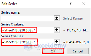
- In the Edit Series dialog box, select X and Y values range of cells.
- In the Y series, we set the normal distribution, in the X series, we set the values.
- Click on OK.
- Add as Series 2 in the Select Data Source dialog box.
- Click OK.
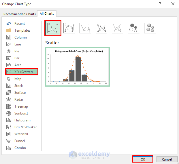
- Go to the Chart Design and Select Change Chart Type from the Type group.
- Select the Scatter type chart. See the screenshot
- Click OK.
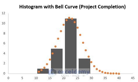
- It will give the bell curve along with the histogram. The curve line is in dotted format.
- We need to make it as a solid line.
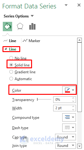
- Double-click the dotted curve, and the Format Data Series dialog box will appear.
- In the Line section, select Solid line.
- Change the Color.
- We have our final histogram result with a bell curve for student marks.
Download the Practice workbook.
Related Articles
- How to Create Probability Histogram in Excel
- How to Add Vertical Line to Histogram in Excel
- Stock Return Frequency Distributions and Histograms in Excel
- How to Create Histogram in Excel Using VBA
<< Go Back to Excel Histogram | Excel Charts | Learn Excel
Get FREE Advanced Excel Exercises with Solutions!

Thank you for the excellent tutorial. It was very helpful. However, I would like to better understand where you got the number 122 in order to scale the curve to the best normal distribution. Do you have any information on how to choose the number for scaling?
Hi ROXANNE,
Thanks for your complement. The number 122 used for scaling is chosen based on empirical or trial-and-error methods to visually match the bell curve with the histogram in the specific context of this tutorial. It is not a standard or universally defined scaling factor; rather, it appears to be chosen to align the bell curve with the histogram in a way that the author finds visually pleasing or appropriate for his dataset. If you are reproducing this analysis for a different dataset, you may need to experiment with the scaling factor to achieve the best visual fit for your specific data. Adjusting this factor allows you to customize the appearance of the bell curve to better match the characteristics of your dataset.
Regards,
Rafiul Hasan
ExcelDemy