How to Summarize Subtotals in Excel (3 Easy Methods)

Summarizing the subtotals in Excel helps us to understand the overall output and group-based output at a time that would take a lot of time if we would calculate individually. We’ll show 3 easy methods in this article to summarize subtotals in Excel with sharp steps and clear illustrations.

Download Practice Workbook

You can download the free Excel workbook from here and practice independently.

What Is Subtotal in Excel?

The subtotal in Excel helps to create different groups according to the dataset. It then allows applying many functions like SUM, COUNT, AVERAGE, MIN, MAX, and other parts to summarize an output. Also, it has the feature to hide or show the summary of any subgroup.

3 Ways to Summarize Subtotals in Excel

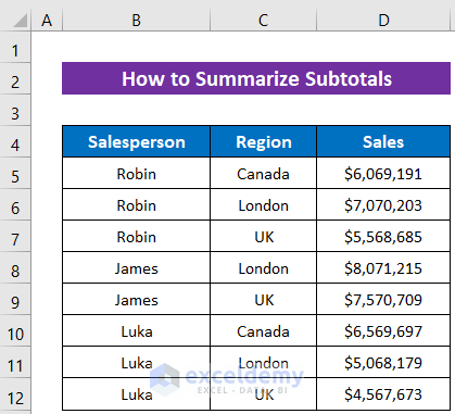
To explore the methods we’ll use the following dataset that contains some salespersons sales in different regions.

1. Applying Subtotal Command to Summarize Data

First, we’ll use the Subtotal command of Excel to summarize the data that you will get in the Outline section of the Data ribbon.

How to Apply Subtotal Command

In this section, we are going to see the way to apply the Subtotal command. Let’s proceed to the procedure.

Steps:

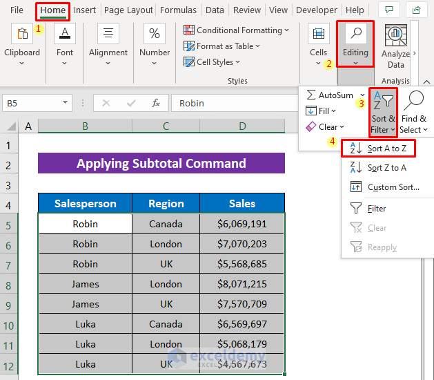
• Before applying the Subtotal command we’ll have to sort the column properly for which you want to find subtotal otherwise you won’t get the output accurately. We’ll find it in the Salesperson column. So select the data range from the column and click as follows: Home > Editing > Sort & Filter > Sort A to Z.

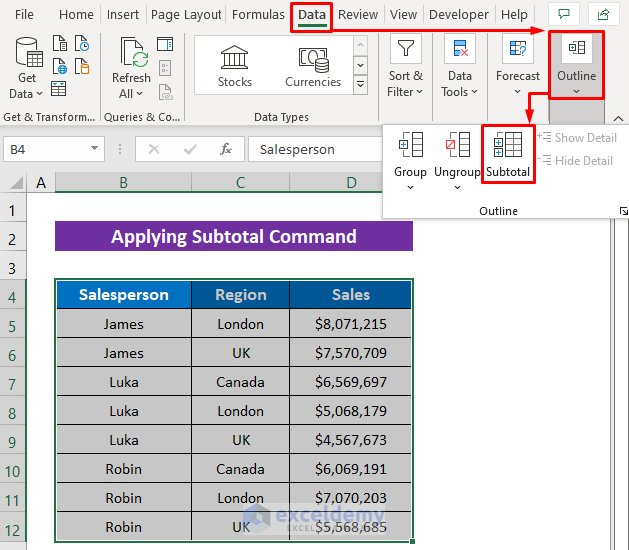
• Then to apply the Subtotal command, click as follows: Data > Outline > Subtotal.

Soon after you will get the Subtotal dialog box.

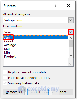
• Next, from the At each change in drop-down box, select the header of the column for which you want to calculate the subtotal.

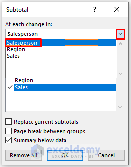
• Later, from the Use function drop-down box select the function which you want to apply to get the subtotal. We’ve selected Sum.

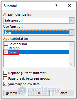
• After that, choose the column where you want to add subtotal.
• Then mark your required option from the three marking options given below in the dialog box.
• Finally, just press OK.

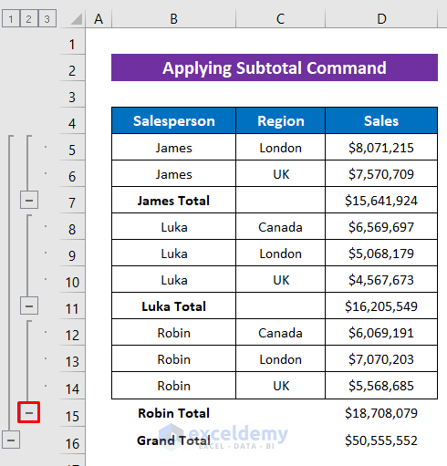
Now have a look, we got the subtotal based on the salesperson column. It grouped our data and showed the total sum for every salesperson. The grouping has 3 layers, the above one is the third layer which shows everything in detail.

• Click on 2 and it will take you to the second layer which will show only every salesperson’s total and grand total.

• After clicking on 1 you will get the 1st layer and that will show only the Grand Total.

Read More: How to Group and Summarize Data in Excel (3 Suitable Ways)

How to Show or Hide Nested Subtotal

You can easily show or hide any nested group from any layer of grouping that will help you to customize your summary.

Steps:

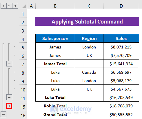
• To hide any group or nested group, just click on the minus sign (-). I hid Robin’s individual sales here.

See, it’s only showing only the Total for Robin.

• To get back it again, click on the plus sign (+).

Soon you will get back the summary then.

Read More: How to Summarize Data by Multiple Columns in Excel

2. Using SUBTOTAL Function to Summarize Subtotals

Now we’ll summarize the subtotal using the SUBTOTAL function. It will allow you to apply a group of functions by an argument k for summarizing data. But the problem is that it can’t make groups like the previous method and had to apply separately for each operation. Here, we’ll find the sum, average, and max value for the summary.

Steps:

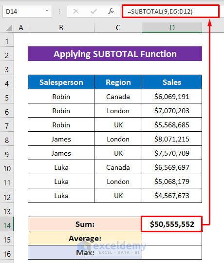
• Insert the following formula in Cell D14, to sum up the grand total-

• Later, just hit the ENTER button for the output.

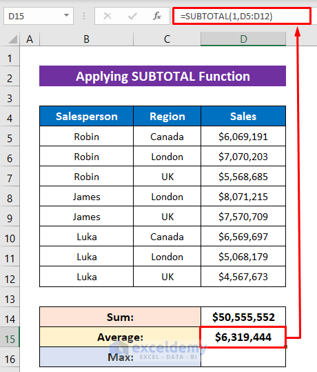
• Then for the average, apply the following formula in Cell D15–

• Press the ENTER button to get the average sales.

• Lastly, to get the maximum sales, type the following formula in Cell D16–

• Hit the ENTER button to finish.

And then you will get the summary like the image below.

Read More: How to Summarize Data Without Pivot Table in Excel

3. Using Excel Status Bar to Summarize Subtotals

There’s another exclusive way in Excel by which you can get the summary of subtotals very quickly at a glance. The lowest bar under the Tab bar is called the Status Bar, whenever you select a data range you will see some summary in the status bar like Average, Count, Sum, etc.

Steps:

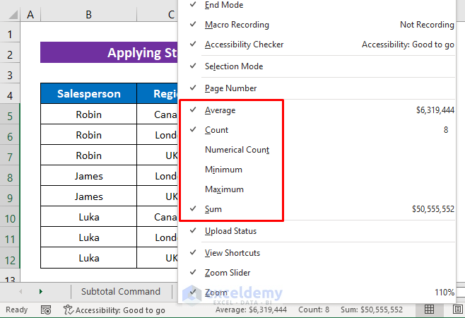
• Just select the data range from your preferred column and then just take a look at the Status Bar and you will get the summary there. My status bar is showing the Average, Count, and Sum.

• By right-clicking on the Status Bar, you can select your required functions from the context menu for the summary.

Read More: How to Create a Summary Sheet in Excel (4 Easy Ways)

How to Remove Subtotal Command

Removing the subtotal command that we applied in the first method is quite easy. Follow the easy procedures step by step.

Steps:

• Select any data from the dataset.
• Next, click as follows: Data > Outline > Subtotal.

• After getting the Subtotal dialog box, just click on Remove All.

Now see, the subtotal operation is removed.

Conclusion

That’s all for the article. Hope the above procedures will be good enough to summarize subtotals in Excel. Feel free to ask any questions in the comment section and give your feedback. Visit our site to explore more about Excel.

Related Articles

• How to Make Summary in Excel From Different Sheets
• Summarize a List of Names in Excel (5 Effective Ways)
• How to Summarize Text Data in Excel (with Easy Steps)
• Summarize Data in Excel Using Pivot Table (2 Examples)
• Linking Excel Sheets to a Summary Page (4 Easy Methods)
• How to Create Summary Table in Excel (3 Easy Methods)