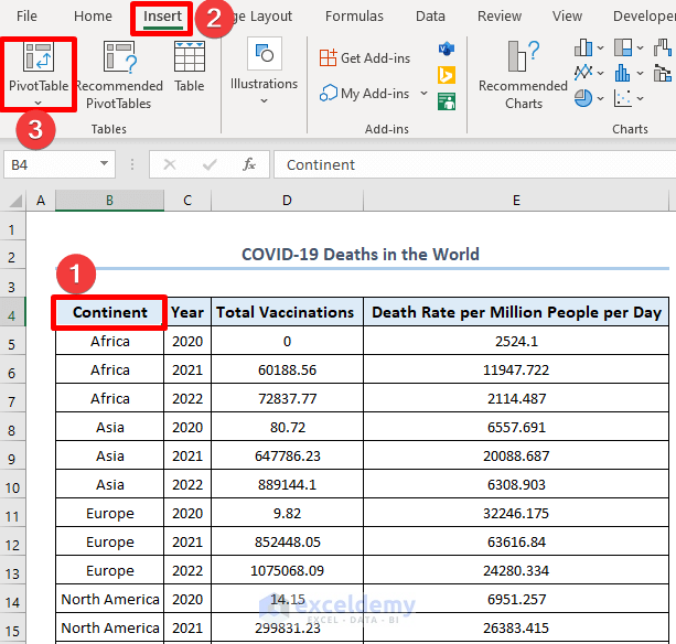
Let’s use a summary of the Covid-19 epidemic between 2020 and 2022 as our sample dataset.

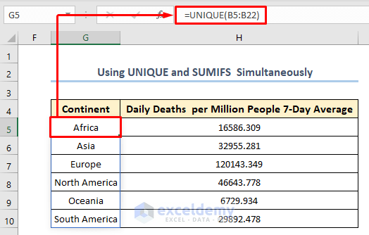
Method 1 – Using UNIQUE and SUMIFS Functions to Create a Summary Table in Excel 365
Steps:
- Use the UNIQUE function and select the whole Continent column. This function lists unique values from the column as an array.
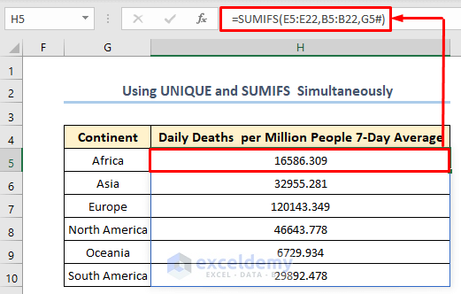
- Use the SUMIFS function and select the column that you want to sum up, the corresponding column to sum up by, in this case, the Continent column, and then the sorted Continent column made from the UNIQUE function.
Read More: How to Summarize Subtotals in Excel
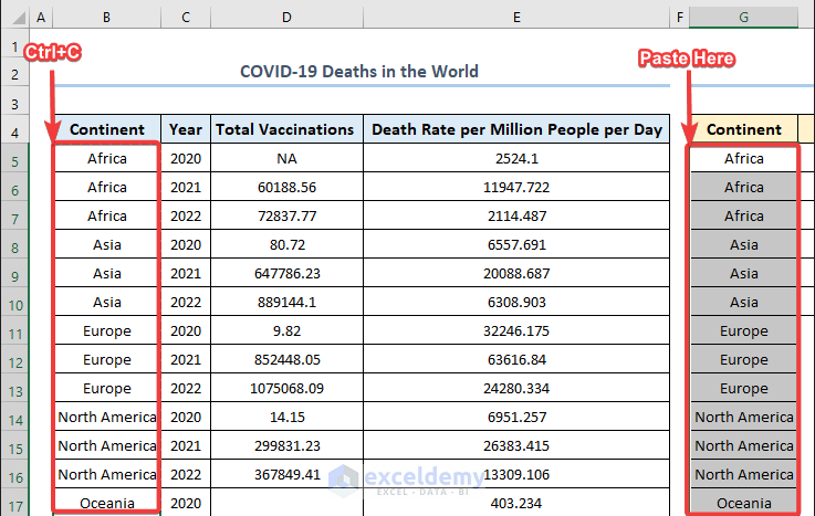
Method 2 – Building a Simple Summary Table Using the SUMIF Function
Steps:
- Copy the Continent column and paste it into the first column of our summary table.
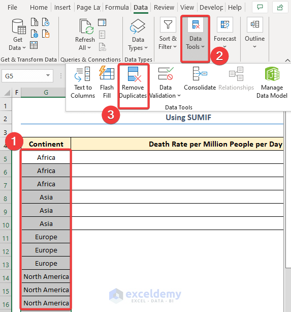
- Remove the repeatedly selected cells by selecting Remove Duplicates under the Data tab.
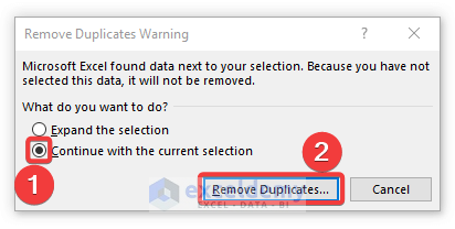
- In the pop-up, select Continue with the current selection and click Remove Duplicates…
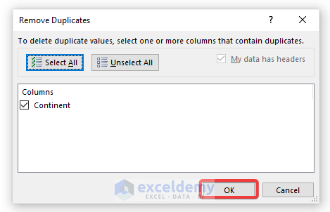
- In the next box, hit the OK button.
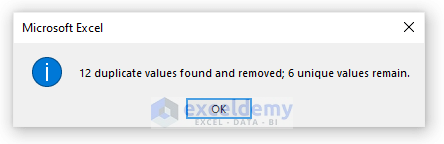
- You’ll get a message box that notifies how many duplicates were removed and how many uniques remain. Click OK.
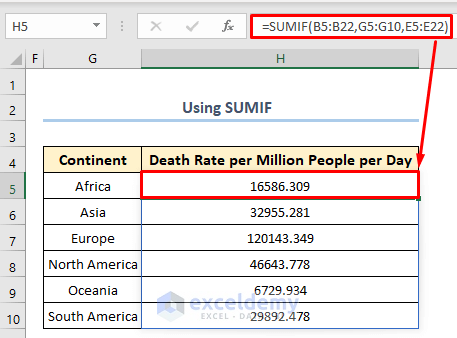
- Type SUMIF in the formula box and select the Continent as the first range, the Continent column in the summary table as the criteria, and the Daily Deaths column as the sum range, in that order.
Method 3 – Using an Excel Pivot Table to Create a Summary Table
Steps:
- Select the table and, from the Insert tab, pick PivotTable.
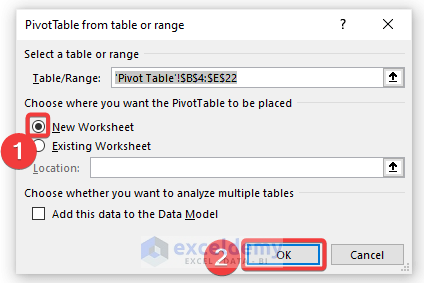
- In the pop-up, click on OK (you may need to choose New Worksheet).
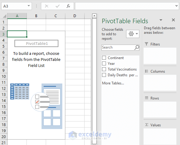
- The PivotTable will be inserted in a new sheet.
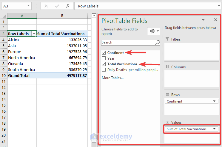
- We have selected Continent and Total Vaccinations, then put Sum of Total Vaccinations in Values. We can also select other options to get an overview of the total dataset.
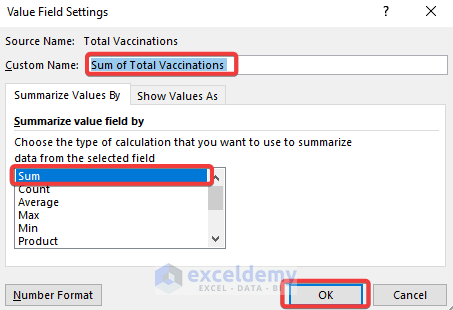
- If you don’t see the Sum option in the Pivot Table Value section, click on the following drop-down.
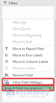
- Select a suitable option from the list.
Read More: How to Create Summary Table from Multiple Worksheets in Excel
Download the Practice Workbook
Related Articles
- How to Summarize a List of Names in Excel
- How to Group and Summarize Data in Excel
- How to Create a Summary Sheet in Excel
- How to Make Summary in Excel From Different Sheets
- How to Summarize Text Data in Excel
- How to Summarize Data by Multiple Columns in Excel
- How to Summarize Data Without Pivot Table in Excel
<< Go Back to Summarize Data In Excel | Data Analysis with Excel | Learn Excel
Get FREE Advanced Excel Exercises with Solutions!

Your information is REALLY helpful BUT please edit the fonts. Those outlined letters are really hard for old eyes.
Hello, Suzette!
Thanks for your appreciation. We will try to use fonts that will be easier to read for old eyes.
Regards
ExcelDemy
this is very helpful for excel master