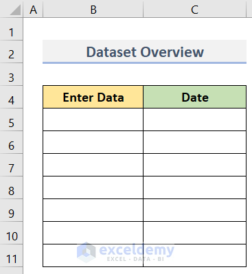
We will put a value in a cell in column B, and the adjacent column C cell will show the date and time of changing the cell.
Method 1 – Applying Excel VBA to Auto-Populate Date When a Cell Is Updated
Steps:
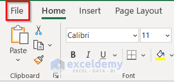
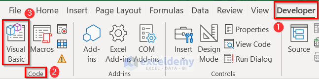
- Check whether your worksheet shows the Developer tab in the ribbon.
- To bring the Developer tab in the ribbon, go to the File tab.
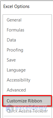
- Choose Options from the left side menu.
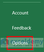
- The Excel Options dialog box will appear.
- Click on Customize Ribbon on the left.
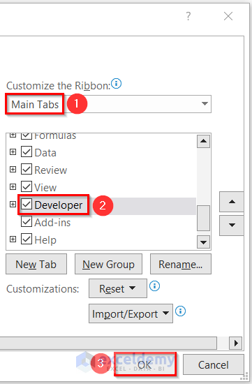
- Choose Main Tabs in the Customize the Ribbon dropdown.
- Check the Developer option in the list.
- Click OK.
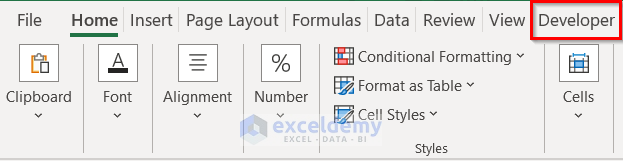
- You should see the Developer tab in the tab list.
- Go to the Developer tab and select Visual Basic.
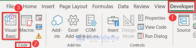
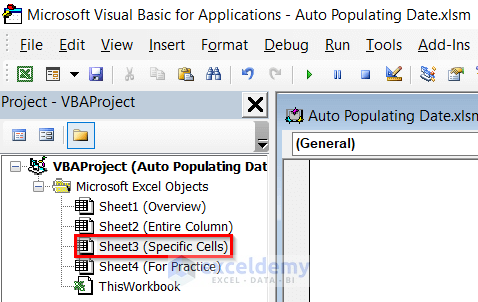
- The Microsoft VBA code editor will open. You can also use the keyboard shortcut Alt + F11 to open this window.
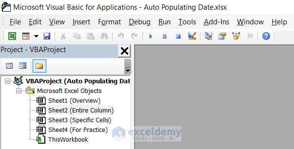
- Double-click on Sheet2 (Entire Column) on the left side of the editor.
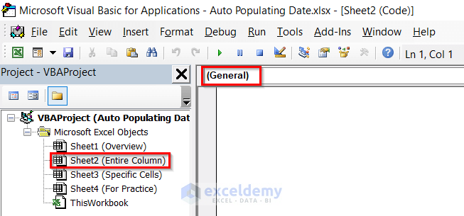
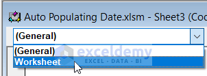
- Click the drop-down part of the (General) and choose Worksheet.
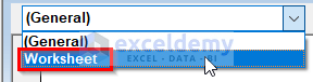
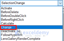
- From the next drop-down, choose the Change option.

- The editor will put two stock functions.
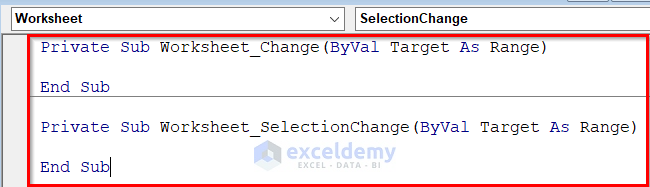
- Select the lower code (see screenshot).
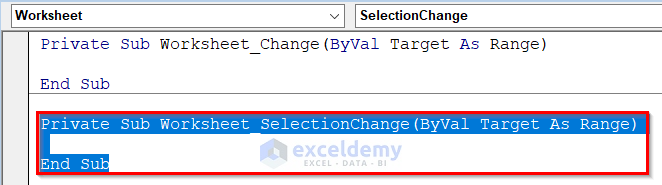
- Press Delete on the keyboard.
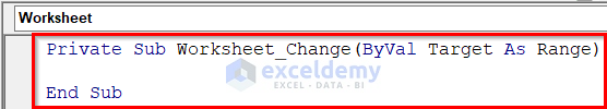
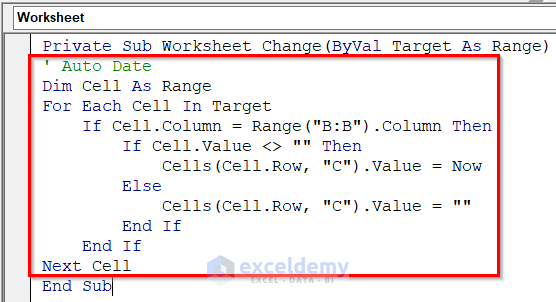
- Insert the VBA code below between the remaining two lines:
' Auto Date
Dim Cell As Range
For Each Cell In Target
If Cell.Column = Range("B:B").Column Then
If Cell.Value <> "" Then
Cells(Cell.Row, "C").Value = Now
Else
Cells(Cell.Row, "C").Value = ""
End If
End If
Next Cell- Here’s the final VBA code.
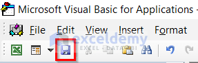
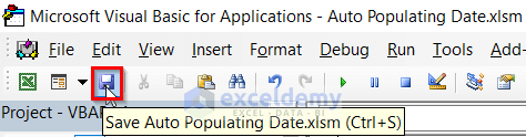
- Click on the Save button located at the upper part of the code window.
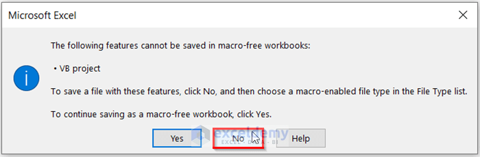
- You may get a notification.
- Select No.
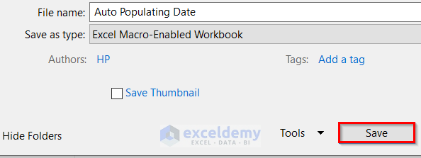
- Choose the Excel Macro-Enabled Workbook option from the Save as type menu.
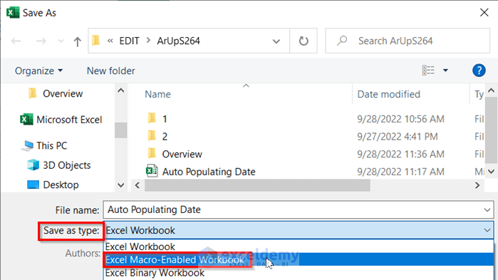
- Click on the Save button to save the new file.
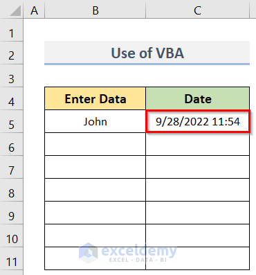
- Return to the worksheet and type anything you want in any cell of column B. We typed John in cell B5.
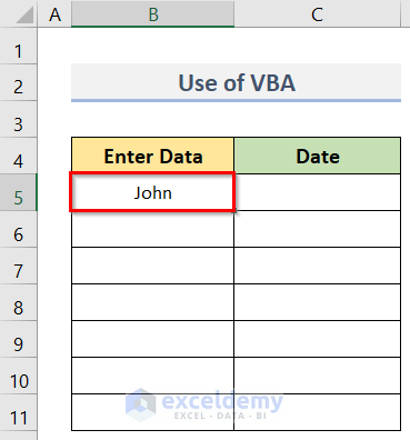
- Press the Enter key and you will get the current date and time in the adjacent cell C5.
- Repeat for other cells of column B.
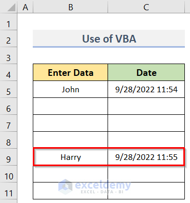
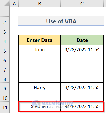
- Here’s our result.
Read More: How to Insert Current Date in Excel
Method 2 – Auto-Populate Date in Excel When a Specific Cell Is Updated
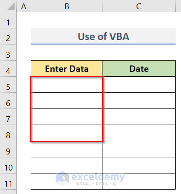
We’ll restrict the function to the range B5:B8.
Steps:
- Go to the Developer tab and click on Visual Basic.
- The VBA code window will appear.
- Double-click on the worksheet named Sheet3 (Specific Cells).
- Select Worksheet from the dropdown of the (General) box.
- Choose Change from the dropdown options of SelectionChange.
- Select the second code in the code window and delete it.
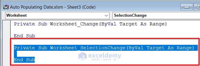
- You should get two lines of code as shown in the screenshot below:
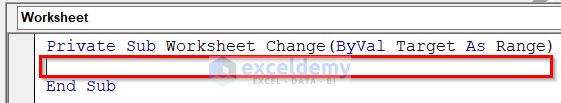
- Insert the VBA code below between the two lines:
With Target
If .Count > 1 Then Exit Sub
If Not Intersect(Range("B5:B8"), .Cells) Is Nothing Then
Application.EnableEvents = False
If IsEmpty(.Value) Then
.Offset(0, 1).ClearContents
Else
With .Offset(0, 1)
.NumberFormat = "dd mmm yyyy hh:mm:ss"
.Value = Now
End With
End If
Application.EnableEvents = True
End If
End With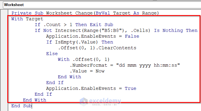
- Click on the Save button in the code window.
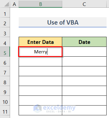
- To check the VBA code, enter any data (Merry) in cell B5.
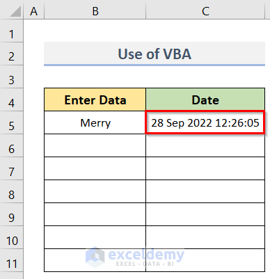
- After pressing Enter, you will get the timestamp in the adjacent cell C5.
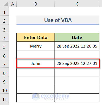
- Enter data in another cell (B7) in the B5:B8 range. You will get the output in the adjacent cell (C7).
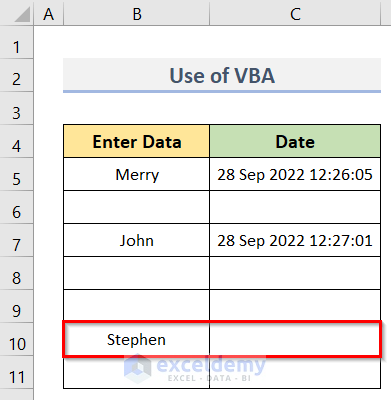
- If you enter data in a cell (B10) out of the range (B5:B8) specified in the VBA code, it will not return any date.
Read More: How to Insert Dates in Excel Automatically
Download the Practice Workbook
Related Articles
- Automatically Enter Date When Data Entered in Excel
- How to Perform Automatic Date Change in Excel Using Formula
- How to Insert Day and Date in Excel
- How to Insert Date in Excel Formula
- How to Get the Current Date in VBA
<< Go Back to Insert Date | Date-Time in Excel | Learn Excel
Get FREE Advanced Excel Exercises with Solutions!

I altered the code to produce different results: Putting the Date in column E and the Time in column F. I am just wondering if there’s a better or shorter way to get this same results?
My revision:
Private Sub Worksheet_Change(ByVal Target As Excel.Range)
With Target
If .Count > 1 Then Exit Sub
If Not Intersect(Range(“D3:D22”), .Cells) Is Nothing Then
Application.EnableEvents = False
If IsEmpty(.Value) Then
.Offset(0, 1).ClearContents
Else
With .Offset(0, 1)
.NumberFormat = “dd mmm yyyy”
.Value = Now
End With
End If
Application.EnableEvents = True
End If
End With
‘Second Function ****
With Target
If .Count > 1 Then Exit Sub
If Not Intersect(Range(“D3:D22”), .Cells) Is Nothing Then
Application.EnableEvents = False
If IsEmpty(.Value) Then
.Offset(0, 2).ClearContents
Else
With .Offset(0, 2)
.NumberFormat = “hh:mm:ss”
.Value = Now
End With
End If
Application.EnableEvents = True
End If
End With
End Sub
I will check out this code. Thanks for the input.
when we normally use as range object we also use set = “something here”. In the very first code above when we declare cell as range we did not use the set keyword. I did not understand why.Can you please explain it to me.
Private Sub Worksheet_Change(ByVal Target As Range)
‘ Auto Date
Dim Cell As Range
Hi Anil,
You are right. We normally use the “Set statement” to assign range objects. But it is done here indirectly without the Set statement.
This is a Change event. Here, “Target” indicates to all cells within the sheet. So the “For Each Cell In Target” statement works as the alternative to the Set statement.
Hope this clarifies your confusion. And thank you for reaching out to us.
Regards
Md. Shamim Reza (ExcelDemy Team)
can I use 2 time stamps in the same excel sheet
input data in column “A” auto date in Column “C”
input data in column “K” auto date in Column “L”
code used:
Private Sub Worksheet_Change(ByVal Target As Range)
‘ Auto Date
Dim Cell As Range
For Each Cell In Target
If Cell.Column = Range(“D:D”).Column Then
If Cell.Value “” Then
Cells(Cell.Row, “B”).Value = Now
Else
Cells(Cell.Row, “B”).Value = “”
End If
End If
Next Cell
End Sub
End Sub
You can check the following code for that. Just copy the ElseIf statement for more columns.
Thanks for reaching out to us. Keep in touch.
Regards
Md. Shamim Reza (ExcelDemy Team)
Hi Kawser.. cool solution.. like your code. Another way to solve this is with a worksheet formula as follows:
=IF(A2=””,””,IF(B2″”,B2,NOW()))
The above assumes your data will go in column A, starting with A2 and the date/time stamp will go in column B, starting with B2. For this to work, you must enable Iterative Calculation in the Options=>Formulas=>Calculations options dialog. Just copy the formula down column B for as far as you want the stamp to work. While VBA can be more flexible, the above is a good way to get it done with a cell formula and an option change. I hope you like it. Thanks again for all of your tutorials.. super helpful and interesting.. makes me better at EXCEL, every time you send them. Thumbs up!
You are most welcome, Wayne Edmondson!
Stay Tuned!
Regards,
Sabrina Ayon
Author, ExcelDemy.
Not sure what happened above to the formula. I think the editor can’t show the less than / greater than symbols. The formula should be:
=IF(A2=””,””,IF(B2 less than symbol and greater than symbol “”,B2,NOW()))
Hope that helps..
Hello, WAYNE EDMONDSON!
Thanks for sharing your thoughts with us!
Stay Tuned!
Regards,
Sabrina Ayon
Author, ExcelDemy.
Is there a way to auto-populate a date based on a specific day rather than current day? For example auto-populate 60 days from August 28, 2019 rather than 60 days from current date?
Thanks for always posting valuable info. I don’t know VBA, but in Excel NOW is volatile. If you insert it as described above, is the date static?
Hello, VICKIE WATT!
Thanks for your comment. Yes, this is date static.
Interested in this same function – but for ROWS vs. columns. We have a shared spreadsheet that needs to be updated by 20+ folks, and want to capture the date ANY TIME a field changes in the ROW. We would allocate column A to be the date field that would get updated if any cell in the row from B:AZ (or however big the range you want). Can’t seem to find this capability.
Hi,
Thanks for this code it is very close to what I am looking for. I need to change the code to capture the date when one of seven different fields is updated. I have changed the range to include all the columns, but it still only works for the first column. Does anyone know what I am doing wrong?
Thanks
Private Sub Worksheet_Change(ByVal Target As Range)
‘ Auto Date
Dim Cell As Range
For Each Cell In Target
If Cell.Column = Range(“J:J”).Column Then
If Cell.Value “” Then
Cells(Cell.Row, “Q”).Value = Now
Else
Cells(Cell.Row, “Q”).Value = “”
End If
End If
Next Cell
End Sub
Great solution perfectly explained Well done sir!
One mod I’m not seeing… I have a short column of cells (B20:B29), which, if one changes, they all change. albeit they may very well hold the same value. Adjacent cells values (C20:I29) will change.
Code works fine however, I only need one date cell currently in B18
Modifying your code in part to read:
If Not Intersect(Range(“B20”), .Cells) Is Nothing Then
Application.EnableEvents = False
If IsEmpty(.Value) Then
.Offset(-2, 0).ClearContents
Else
With .Offset(-2, 0)
changes the date in that cell, but only if attributed to B20 else it overwrites successively the values in B .Offset(-2, 0).
I’m not so clever in VB I can figure out a solution.
Any offers?
Hi Kawser,
Great code for udating the date.
One thing that I would like to see (how to do it) is to have the date change every time the adjacent cell changes.
Some 4500 rows of data and the status column (lets say N:N) can change between 5 different listings. I do use the Filter Function to generate a report, however, if the date is changed by VBA (my code) the #Spill will not occur in the report sheet. Adding the date manually allows the SPILL.
My code I have is:
Private Sub Worksheet_Change(ByVal Target As Range)
‘Auto Date input when adjacent cell changes.
Dim xCellColumn As Integer
Dim xTimeColumn As Integer
Dim xRow, xCol As Integer
Dim xDPRg, xRg As Range
xCellColumn = 14
xTimeColumn = 15
xRow = Target.Row
xCol = Target.Column
If Target.Text “” Then
If xCol = xCellColumn Then
Cells(xRow, xTimeColumn) = Now()
Else
On Error Resume Next
Set xDPRg = Target.Dependents
For Each xRg In xDPRg
If xRg.Column = xCellColumn Then
Cells(xRg.Row, xTimeColumn) = Now()
End If
Next
End If
End If
End Sub
Just hoping someone may know the answer.
Cheers
Hi Greg,
That is really good input from you. Hope your piece of code will help people who are in trouble. Cheers!
Best regards
Thanks for this code!
When I run it the date isn’t input into the adjacent cell until I go back up to the cell.
Do you know any fix for this?
How do you add multiple codes for the same sheet? I want to auto-date multiple columns, not just 1.
Hi,
when im closing the file and open it again, the function is not working.
you know maybe why ?
i saved it as enabled workbook
The only thing I don’t like about this is that “undo” no longer works on the cells that are being monitored. Is there any way to change that?? Otherwise, this was very helpful, thank you. As info: For my specific needs, I wanted to check multiple columns, so I just repeated the first solution. Not at all elegant but it worked. Also, I didn’t want the date to get deleted if a cell changed back to empty, so I changed the ELSE result to also be = Now.
Like this:
Private Sub Worksheet_Change(ByVal Target As Range)
‘ Auto Date column L if any cell in columns B thru K are modified
Dim Cell As Range
For Each Cell In Target
If Cell.Column = Range(“B:B”).Column Then
If Cell.Value “” Then
Cells(Cell.Row, “L”).Value = Now
Else
Cells(Cell.Row, “L”).Value = Now
End If
End If
Next Cell
For Each Cell In Target
If Cell.Column = Range(“C:C”).Column Then
If Cell.Value “” Then
Cells(Cell.Row, “L”).Value = Now
Else
Cells(Cell.Row, “L”).Value = Now
End If
End If
Next Cell
For Each Cell In Target
If Cell.Column = Range(“D:D”).Column Then
If Cell.Value “” Then
Cells(Cell.Row, “L”).Value = Now
Else
Cells(Cell.Row, “L”).Value = Now
End If
End If
Next Cell
End Sub
Thanks a lot of your input, Andy!
Is there a way to implement this without the timestamp being included in the date? Not just formatting, just in the formula bar as well.
Hello ABBY!
You have to change a line in the VBA code that is defining the format of the output.
Insert this line:
.NumberFormat = “dd mmm yyyy” instead of this .NumberFormat = “dd mmm yyyy hh:mm:ss”
So, the code will become as follows-
Good explanation. Thanks.
However, I should like to adapt this to get the dates in a row instead of in a column.
Would appreciate any suggestions. Thanks.
Hello ARIF, to get the dates in the next row use the following code when you will insert values in cells of range B3:I3 and want to auto-populate date and time in cell range B4:I4.
CODE:
You can change the cell range as your want. I hope, your problem will be solved in this way. If not, please share the Excel file and send us the problem with a little more explanation in an email at [email protected]
How can you edit this code to check 3 columns or more for data entry instead of the 1?
Hi
You can check the following code for that. Just copy the ElseIf statement for more columns.
Thanks for reaching out to us. Keep in touch.
Regards
Md. Shamim Reza (ExcelDemy Team)
Hello,
I am following the auto date. I am just wondering how do I do it if I would like another column to act the same.
For example, I fill out Column C with data, and Column B will automatically update with the date when Column C was filled out.
How will I do it if I would like to have Column E to automatically update with the date and time when I fill Column D with “Delivered”
I hope it does make sense. I tried following some pointers here and putting two and two together. But I can’t seem to make it work. Thanks so much!
Hello, GIA!
As you mentioned, you fill out Column C with data, and Column B will automatically update with the date when Column C was filled out. All you need to do is change the range in your code, and also change the reference argument which is the offset. Try this code below.
Also, you can use the same code for column E to automatically update with the date and time when you fill Column D with “Delivered”. You just have to change the range.
Please follow the instructions of the method I linked down.
https://www.exceldemy.com/auto-populate-date-in-excel-when-cell-is-updated/#2_Auto_Populate_Dates_in_Some_Specific_Cells_While_Updating_with_Excel_VBA
Hope this will help you!
Best Regards.
I am using this code for auto dating, I am trying to add a way to lock down the row so no changes can be made after they sign and it provides the date.
Dim Cell As Range
For Each Cell In Target
If Cell.Column = Range(“G5:G300”).Column Then
If Cell.Value “” Then
Cells(Cell.Row, “E”).Value = Now
Else
Cells(Cell.Row, “E”).Value = “”
End If
End If
Next Cell
I am trying to add coding that will lock the row after the date auto updates. Then I want it to create an audit log onto another sheet.
Dim Cell As Range
For Each Cell In Target
If Cell.Column = Range(“B:B”).Column Then
If Cell.Value “” Then
Cells(Cell.Row, “C”).Value = Now
Else
Cells(Cell.Row, “C”).Value = “”
End If
End If
Next Cell
Hello, JOHN!
Thanks for your comment!
You can lock the row after the date auto updates with the following code.
A cell should only be locked if cell A1 was updated and it is not blank, according to this formula: if Target.Address = “$A$1” and Target.Value > “”
Just substitute the relevant cell value for $A$1 to make the macro function on cell B1, cell D15, or any other cell. For this to function, the column and row references must be preceded by dollar signs.
By changing > “” in the line above to = “desired value,” you may additionally lock the cell only if a certain value was entered, allowing you to do things like lock the cell only if OK was entered or anything similar.
Hope this will help you!
Good Luck!
Regards,
Sabrina Ayon
Author, ExcelDemy.
Hello,
I am working with this codes for my project for a while, and I am able to make some work, the way I like it to. However, what I am trying to achieve is this.
Column D will have updatable information like stages in an entire process. Ex. “Start” “In-Progress”, “Pending”, “Completed”, and so on.
What I want to happen is have the Dates for each stages will be stamped on different columns. For example,
When Column D is set to “Start”, Column G will have the date, then if Column D is updated to “In-Progress” Column H will have the date… so on and so forth.
Thanks so much!
Hi,
Thank you for your comment. From the problem you have stated, it looks like you need to just modify the previous code a little bit. You can use the following code to accomplish your task.
Regards,
Md. Abu Sina Ibne Albaruni
Team ExcelDemy
I have a similar problem I am trying to solve, but don’t see that it’s been asked. I have a spreadsheet with 400 rows and want to have column N automatically update with today’s date when anything is changed in the row for columns O:V.
Thank you Heidi for your comment. You can paste the following VBA code into your Desired Worksheet on the VBA window. This code will automatically update the current date in the corresponding cell of column N if anything is changed in columns O:V. Hope, it will solve your problem. If you have any further queries, you can post them on our Exceldemy Forum.
Regards
Aniruddah
Team Exceldemy
How would I write this so that when data is entered into column C date populates in Column A and time populates in column B?
Hello JEREMY,
Thank you for your comment. I’ve understood your problem. You can use the following instruction. Don’t paste this code into the module. Use it in the sheet module.
Right-click on the sheet name and select the View Code option from the context menu.
Besides, you can double-click on the specific sheet to add a module for this sheet especially.
In the module, paste the following code.
You don’t have to run this code. Simply, save it and return to the worksheet and it’ll work smoothly.
If you delete the data in Column C, the date and time for this particular data will be erased also. But, don’t delete the entire column, it’ll create an error and you have to press CTRL + X to stop the macro from running.
Again, thanks for your query. We always welcome our readers to ask this type of info-ful questions.
Regards,
SHAHRIAR ABRAR RAFID
Team ExcelDemy
Hi! I am trying to auto fill a cell yellow anytime a change is made to the data inside the cell. Could I use a form of this code to achieve this? THIA!
Hello NIKKI
Thanks for reaching out and sharing your queries. You want to automatically fill a cell background to yellow anytime a change is made to the data inside the cell.
I am delighted to inform you that I have developed an Excel VBA change event that will fulfil your goal. To demonstrate, assume you want to auto-fill a cell in column A to yellow.
To do so, open the sheet module => Insert the following code and Save.
Now, return to the sheet and change some cell values in column A to get an output like the following GIF.
Hopefully, the idea will help you. Good luck.
Regards
Lutfor Rahman Shimanto
Excel & VBA Developer
ExcelDemy
Thank you for this thread, it has been really helpful. My only issue is the “undo” function no longer works on the cells being monitored. Has anyone found a way around this please?
Hello Adele
Thanks for your nice words. We are glad you found the article helpful!
In Excel, we are directly unable to undo a VBA macro action in the same way you can undo regular actions using the Ctrl + Z shortcut. So, you must use the Excel Track Changes feature, or you can also use external version control systems like Git.
I hope these ideas will overcome your situation; good luck.
Regards
Lutfor Rahman Shimanto
ExcelDemy