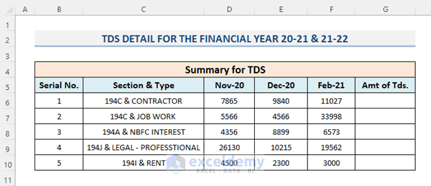
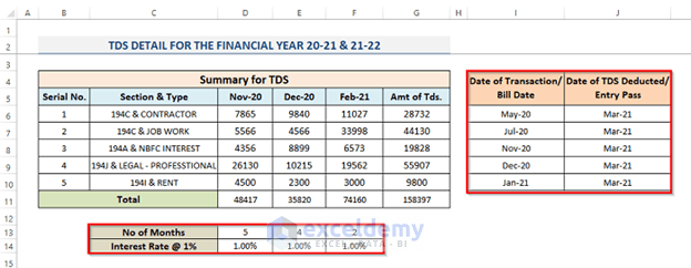
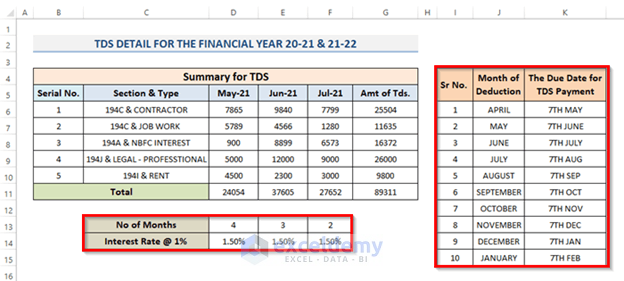
How to Create TDS Interest Calculator in Excel: 9 Methods

Method 1 – Summary of TDS for Late Deduction

We record all the sections and type in column C and TDS statement for the month of November, December and February.

tds interest calculator excel

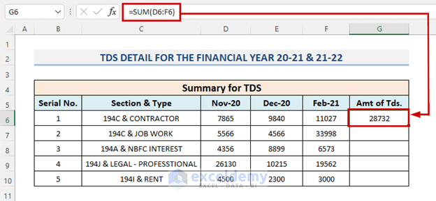
Select a cell to calculate the amount of TDS. For this, we will use the SUM function. The SUM function is used to add values.
Select the cell where we want to see the result and insert the formula of SUM function.

=SUM(D6:F6)

Press the Enter key from your keyboard.

tds interest calculator excel

To duplicate the formula over the range or Auto-Fill the range, drag the Fill Handle icon down or double-click on the plus (+) symbol.

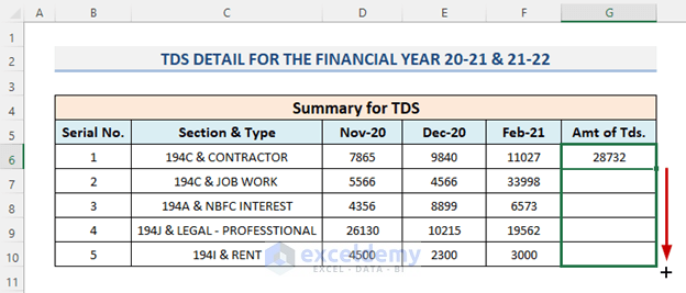
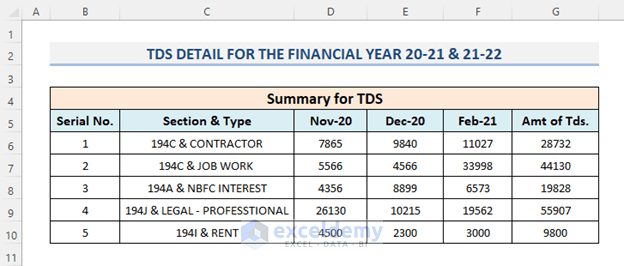
See that the result of the TDS amount will show in column G.

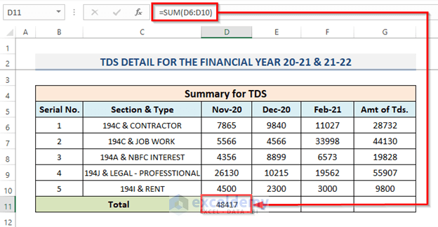
Calculate the total of individual TDS statements as well as the total TDS amount. So, first we will compute this for November-20. So, we select cell D11 and put the formula into that cell.

=SUM(D6:D10)

Hit Enter to see the result.

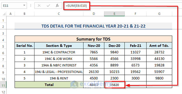
Calculate the total of December-20’s TDS.

=SUM(E6:E10)

Press Enter.

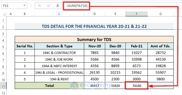
For the month of February-20, we will use the SUM function.

=SUM(F6:F10)

Hit the Enter key.

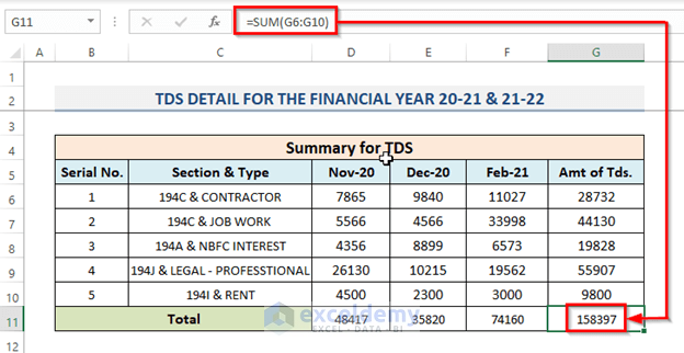
Compute the total TDS amount.

=SUM(G6:G10)

Hit Enter to see the result.

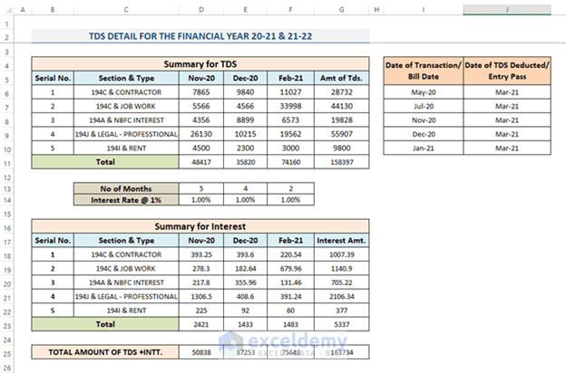
Method 2 – Input Necessary Information

The number of months and the interest rate.
We will list the Date of Transaction or Bill Date along with the Date of TDS Deducted or Entry Pass.

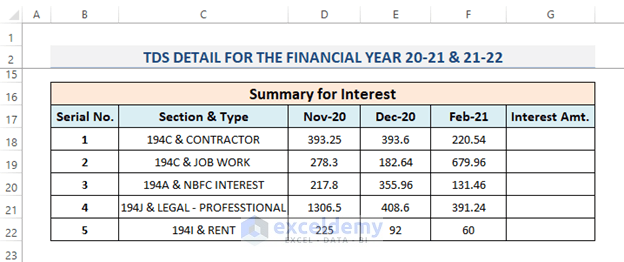
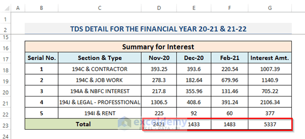
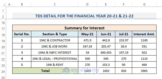
Method 3 – Summary of Interest for Late Deduction

The previous step, first, we record every part and enter the TDS statement for November, December, and February in column C.

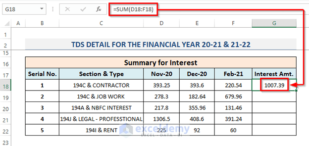
Choose a cell and calculate the TDS in that cell. We’ll employ the SUM function for this.
Choose the cell where we want to view the outcome. Add the SUM function formula after that.

=SUM(D18:F18)

Press the Enter key on your keyboard once more.

To copy the formula over the range, drag the Fill Handle symbol downward. Double-click the addition (+) sign to AutoFill the range.

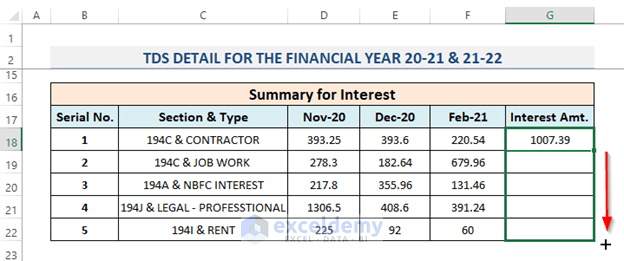
Compute all the totals, as we compute the totals at the first step.

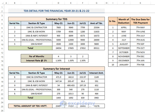
Method 4 – Calculate Total Amount

Select the cell D25 and put the formula of addition into that selected cell to compute the total for the month of November.

=D11+D23

Press Enter.

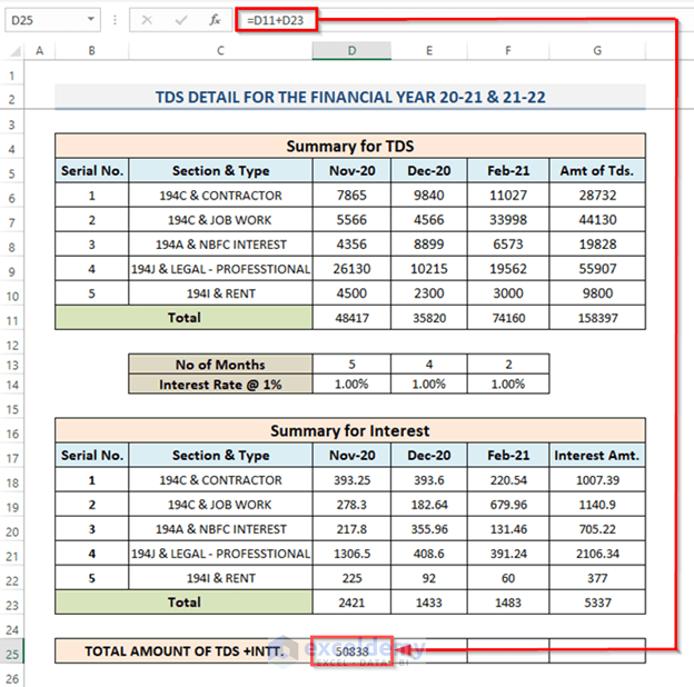
Compute the total for December and February. Also for the total of TDS and interest using the additional formula.

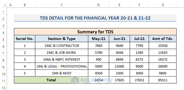
Method 5 – Encapsulation of Late Deposit

Begin with, likewise, the summary of late deduction, we will record all the sections and type also the months.
The amount of TDS using the SUM function.
The total of all the individuals.

Method 6 – Enter the Required Information

Consider the interest rate and the number of months.
In addition to the Month of Deduction, we will also give the Due Date for TDS Payment.

Method 7 – Condensation of Late Deposit

As with the late deduction summary, we will first list all the sections and type the months.
Using the SUM function, add the TDS quantity as well.
The total of each individual is shown last.

Method 8 – Determine Total Amount

Select the required cell and put the formula of addition into that selected cell.

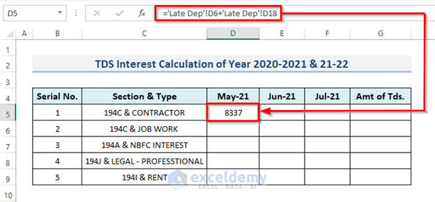
Method 9 – Precis TDS Interest Calculator

Select the cell where we want to put the result. In our case, we will choose cell D5.
Insert the formula into that cell.

=’Late Dep’!D6+’Late Dep’!D18

Press Enter key from the keyboard.

Drag the Fill Handle icon to copy the formula over the range. You can also double-click on the plus (+) sign to duplicate the formula.

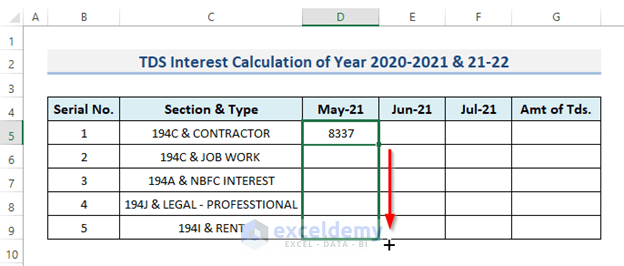
Following the month of May-21, do the same for other months.

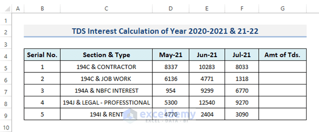
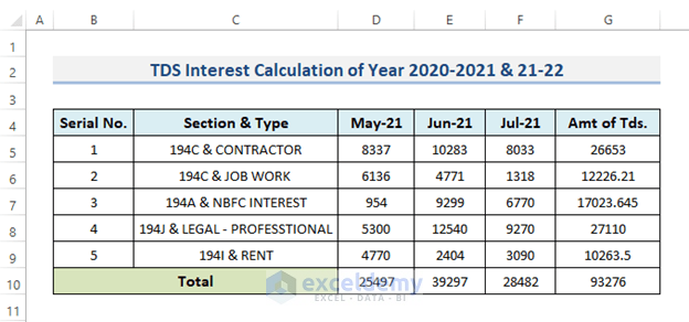
Compute the amount of TDS. We will use the SUM function. The SUM function is a built-in function, categories under the Math/Trig Function. This adds each value in a range of cells before returning the total.
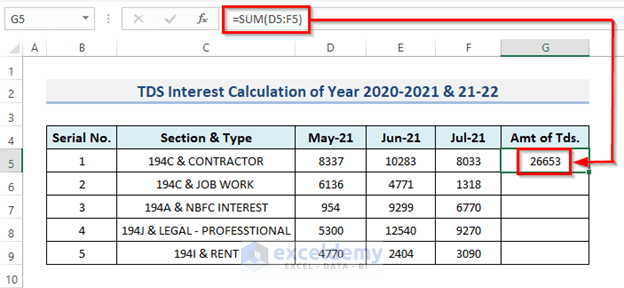
Select the second cell G5, and put the formula into that selected cell.

=SUM(D5:F5)

Hit the Enter key to see the outcome.

Drag the Fill Handle icon down to duplicate the formula over the range. To Auto-Fill the range, double-click on the plus (+) symbol.

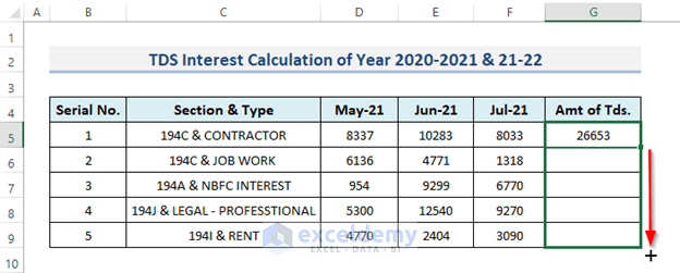
The calculator is ready to use. If we change any data from the Late Deb and Late Dep sheets, this will automatically change the calculator data.