How to Create an Accrued Interest Calculator in Excel – 5 Methods

Download Practice Workbook

Download the Excel workbook and practice.

What Is Accrued Interest?

The Accrued Interest is interest that has been incurred on financial transactions but has not yet been paid out. Investors regard it as profit.

Face Value                  = Initial Price of the Bond
Daily Interest Rate     =Annual interest/365
Days                            =Last Issue date- Settlement date

Method 1 – Calculating Accrued Interest Manually

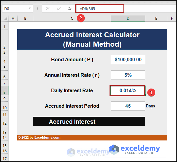
You have a bond amount and an annual interest rate. To calculate accrued interest on this bond:

Steps:

• Select D8 and enter the following formula.

D6 represents the Annual Interest Rate. 365 indicates the total days in a year.

• Press ENTER.

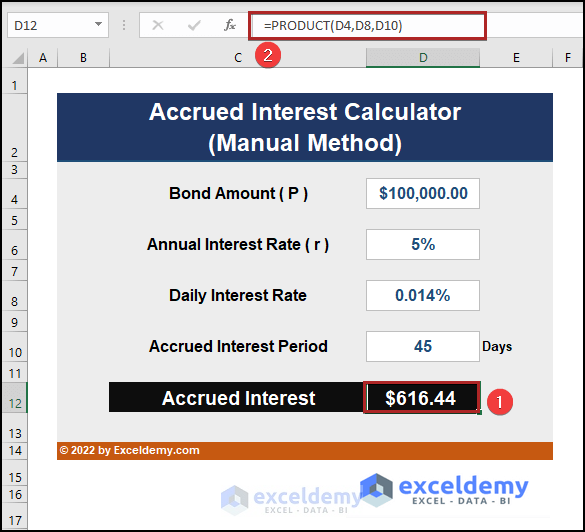
• Go to D12 and enter the formula below.

The three entities are multiplied using the PRODUCT function.

• Press ENTER.

• Alternatively, use the following formula in D12.

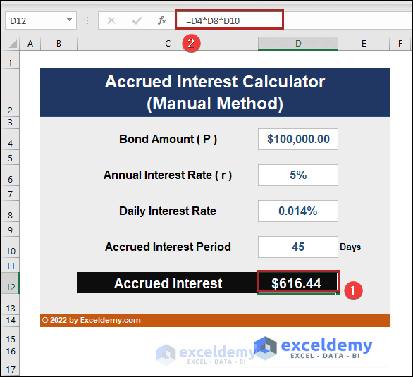
The accrued interest for the amount of $1,00,000 on a 5% annual interest rate for a period of 45 days is $616.44.

Read More: How to Create Monthly Accrued Interest Calculator in Excel

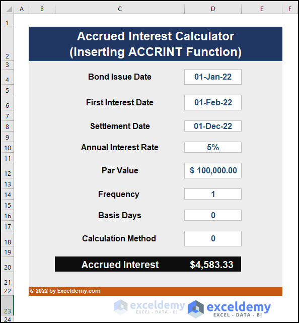
Method 2 – Using the ACCRINT Function

The formula for the ACCRINT function is:

issue: the date when a loan or bond is issued.
first_interest: the date when the interest payment will first occur.
settlement: the date when the loan will be finished.
rate: annual or yearly Interest rate.
par: The bond/loan amount.
frequency:  the annual number of loan payments. 1 for Annual payments, 2 for Semi-annual payments, and 4 for Quarterly payments.
basis:  is set to 0 if the argument is omitted. [Optional]
0 Or Omiited- US (NASD 30/360)
1– Actual/Actual
2– Actual/360
3– Actual/365
4-European 30/360
calc_method: It’s either 0 or 1 (calculates accrued interest from first_interest date to settlement date). [Optional]

Steps:

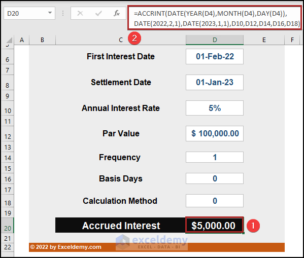
• Select D20 and enter the following formula.

• Press ENTER.

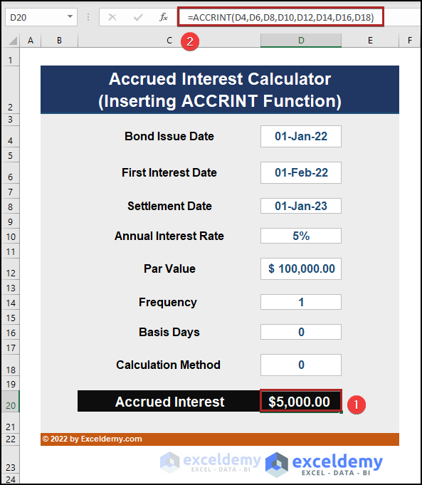
The accrued interest amount is $5000 for 12 months from January 22 to January 23.

Interest is calculated by multiplying C10 by C12:  $5000.This value is divided by 12 as the basis is 0: $416.67. $416.67 is multiplied by 12 (months).

• If you change the Settlement Date to 1 Dec 2022 this is the output.

The interest amount is $4583.33 (11 months): $416.33 * 11 = $4583.33.

Read More: Create Late Payment Interest Calculator- Download for Free

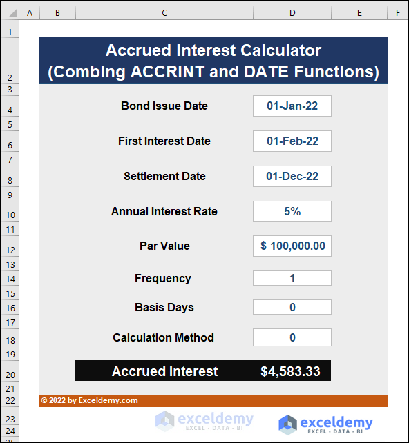
Method 3 – Combining the ACCRINT and the DATE Functions

Use the ACCRINT and the DATE functions to change the date format.

Steps:

• Select D20 and enter the following formula.

To use the cell reference apply the DATE and the YEAR, MONTH, and DAY functions.

• Press ENTER.

For 11 months the amount is: $4583.33.

Read More: How to Create FD Interest Calculator in Excel

Method 4 – Using the DAYS360 Function

The DAYS360 function considers every month as 30 days and the whole year as 360 days. The syntax of the function is:

Steps:

• Select D16 and use the following formula.

• Press ENTER.

The accrued interest for 1 month from Dec 22 to Jan 23 is displayed.

Read More: How to Make TDS Interest Calculator in Excel

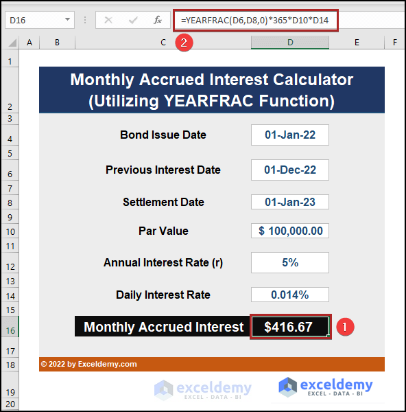
Method 5 – Utilizing the YEARFRAC Function

The YEARFRAC function represents the fraction value of the year calculating the difference between two dates. The syntax of the function is the following:

You must multiply the returned value by 365, Par Value, and Daily Interest Rate to display the accrued interest.

Steps:

• Go to D14 and use the formula below.

• Press ENTER.

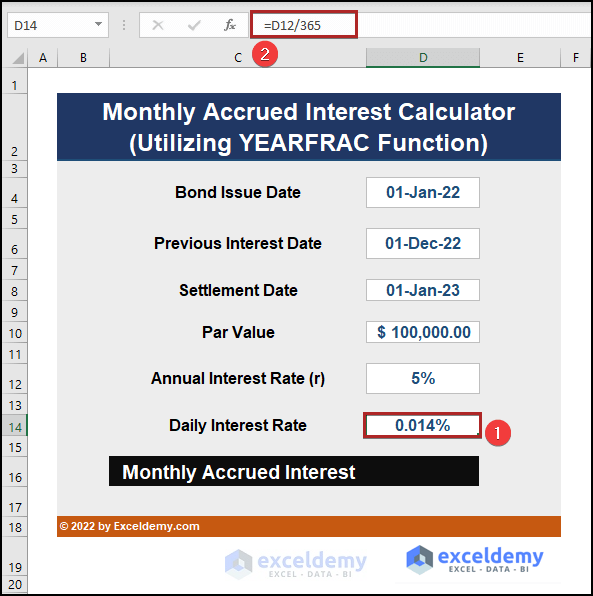
• Select D16 and enter the following formula.

• Press ENTER.

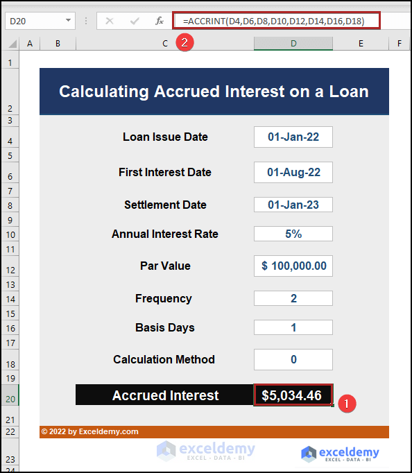
How to Calculate Accrued Interest on a Loan

Like in Method 2, you can use the ACCRINT function to calculate accrued interest on a loan.

Steps:

• Go to D20 and enter the formula below.

• Press ENTER.

Read More: How to Create TDS Late Payment Interest Calculator in Excel

Things to Remember

• In the U.S., 30/360  is used for corporate and municipal bonds. U.S. Treasury notes and bonds use the actual/actual day count basis.
• Only the ACCRINT formula accurately returns accrued interest.
• The arguments for the first_interest date and settlement date should be valid dates.

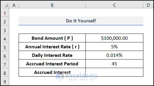
Practice Section

Practice here.

Related Articles

• Create a Post-Judgement Interest Calculator in Excel
• How to Create a Money Market Interest Calculator in Excel
• How to Generate GST Interest Calculator in Excel
• Make Service Tax Late Payment Interest Calculation in Excel
• Create a Simple Interest Loan Calculator with Excel Formula

<< Go Back to Finance Template | Excel Templates