How to Create Money Market Interest Calculator in Excel

In this article, we will present 4 easy steps to create a money market interest calculator in Excel. We also provide a free template at the bottom.

What Is the Money Market?

A money market fund is a kind of short-term investment. “Money” refers to a variety of assets that can be quickly converted into cash, such as short-term government securities, bills of exchange, or bankers’ acceptances. The money market entails huge overnight cash transfers between banks and the government, and the vast majority of money market transactions are wholesale exchanges between businesses and financial institutions. Many financial institutions such as banks offer the opportunity to invest in Money Market Funds, paying interest in return for the liquidity provided.

4 Steps to Create Money a Market Interest Calculator in Excel

Let’s create a money market interest calculator to calculate how much interest we’ll earn from a money market fund investment.

Step 1 – Create the Basic Outline

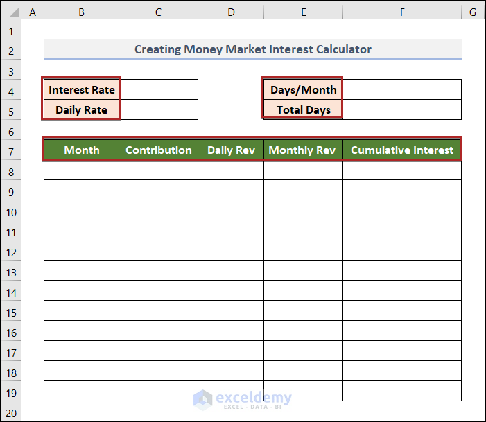
First of all, we’ll construct a basic outline in which all the information will be placed.

Build an input range in cells C4:C5. Insert the Interest Rate manually. We’ll calculate the Daily Rate automatically a bit later.
In the F4:F5 range, create an input area for the Total Days in a year and the number of Days/Month.
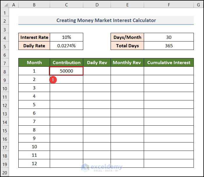
In the last table, insert headings as in the image below.
- For the number of Months, if we make a deposit at the start of a month, this will be month 1, the next month will be month 2, and so on.
- The heading Contribution means the initial deposit made at the start of the investment.
- Daily Rev means the daily earnings from the interest.
- Multiplying Daily Rev by the number of days per month gives us the Monthly Rev.
- Finally, Cumulative Interest means the total running interest, or the amount of interest including previous months.

Step 2 – Determine the Daily Interest Rate

As a money market fund is a short-term investment, the interest is calculated on a daily basis because the interest rate changes daily. Let’s calculate the daily interest rate.

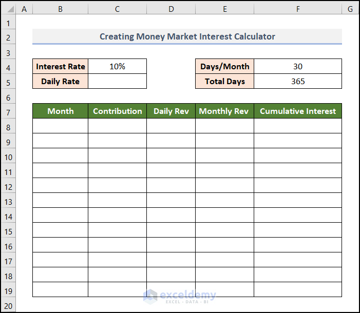
Assume an annual Interest Rate of 10%, 30 days per month and 365 total days in a year.

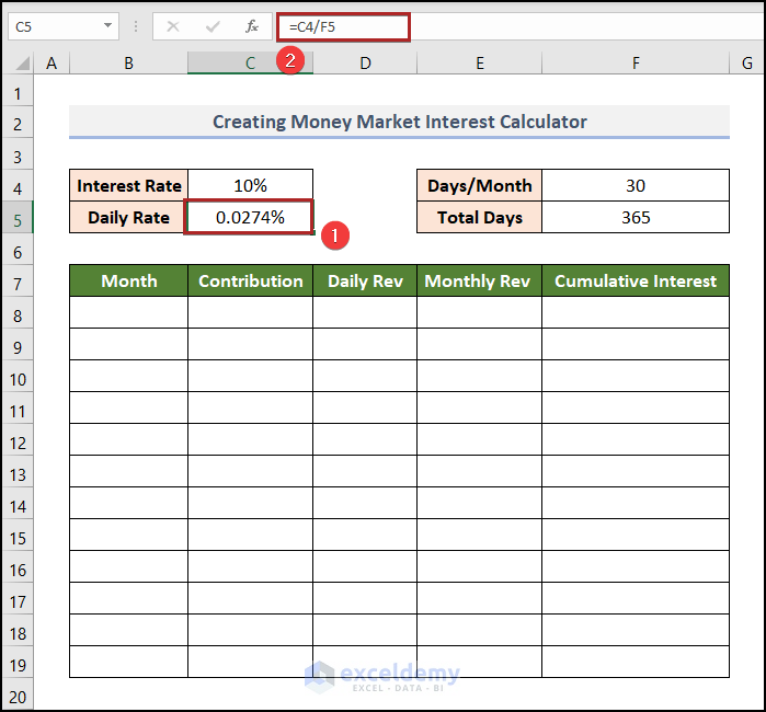
To calculate the Daily Rate from this information:

In cell C5, enter the following formula:

=C4/C5

So, we divide the annual interest rate by the number of days in a year, 365, to get the daily rate of interest.

Press ENTER.

Step 3 – Calculate the Daily and Monthly Revenue

Next, we’ll compute the daily earnings as well as the monthly income from the investment.

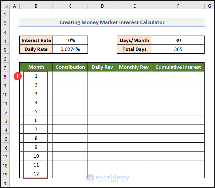
Enter the number of months in order in the Months column.

Enter the initial deposit amount in cell C8. In this case, we put 50,000.

In cell D8, enter the formula below:

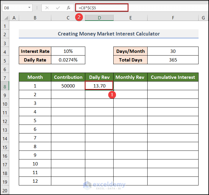
=C8*$C$5

We multiply the deposit amount in cell C8 by the daily interest rate in cell C5 to get the Daily Rev.

Press ENTER.

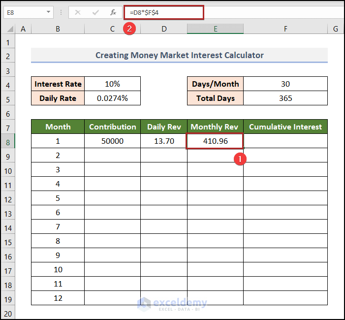
In cell E8, enter the following formula:

=D8*$F$4

We multiply the Daily Rev in cell D8 by the number of Days/Month in cell F4 to get the Monthly Rev.

Press ENTER.

Step 4 – Calculate the Total Running Interest

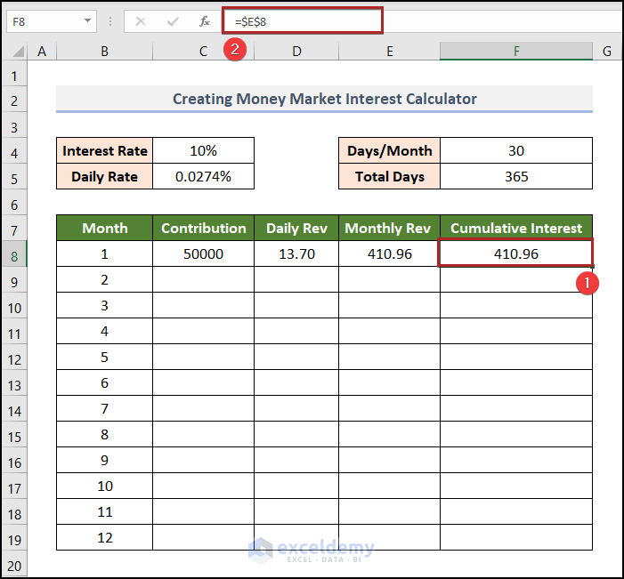
In the last column, we’ll calculate the cumulative interest. In the first month, it’s different from the other months.

In cell F8, enter the following formula:

=$E$8

The initial value is an absolute reference to the corresponding Monthly Rev from cell E8.

Press ENTER.

To calculate the second month’s cumulative interest:

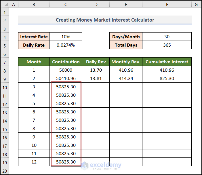
In cell C9, enter the following formula:

=C8+E8

The second month’s value is the monthly revenue of the previous month in cell E8 plus the deposit amount in cell C8.

Press ENTER.

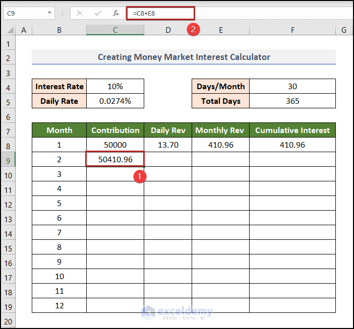
Note: The interest amount for the second month will be calculated based on this amount in cell C9.

Calculate the Daily Rev and Monthly Rev just like in Step 3.

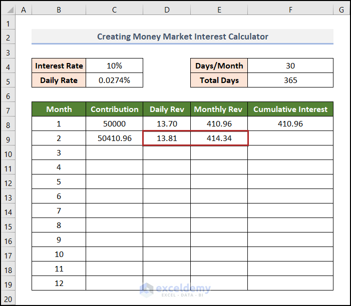
Now we can determine the cumulative interest amount for the second month.

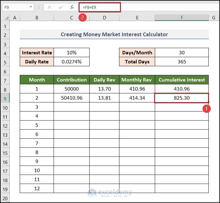
In cell F9, enter the following formula:

=F8+E9

The cumulative interest is the sum of the interest for the current month in cell E9 and the previous month’s cumulative interest in cell F8.

Press ENTER.

Double-click on the Fill Handle.

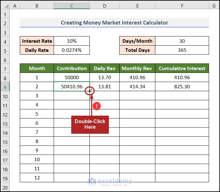
The remaining cells in this column are filled automatically.

Note: The results shown are incorrect now. However they will be correct after the completion of the task.

Repeat the process for columns D, E, and F.

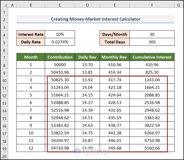
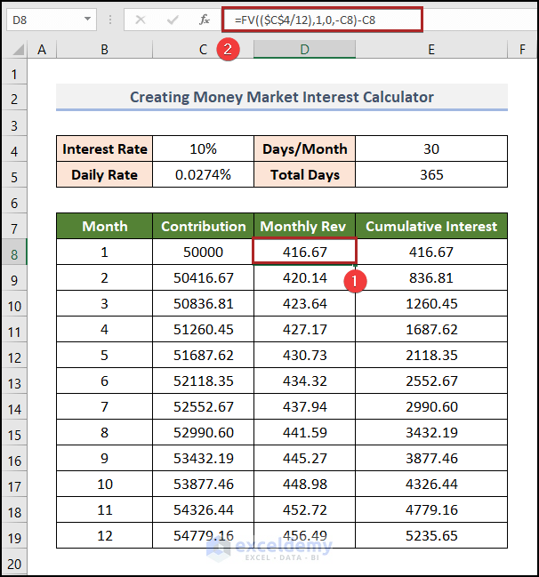
Our table is completely filled. The amount in cell F19 is the final amount of interest gained from the money market account after a year.

We can get a more accurate result using the FV function, as in the mage below.

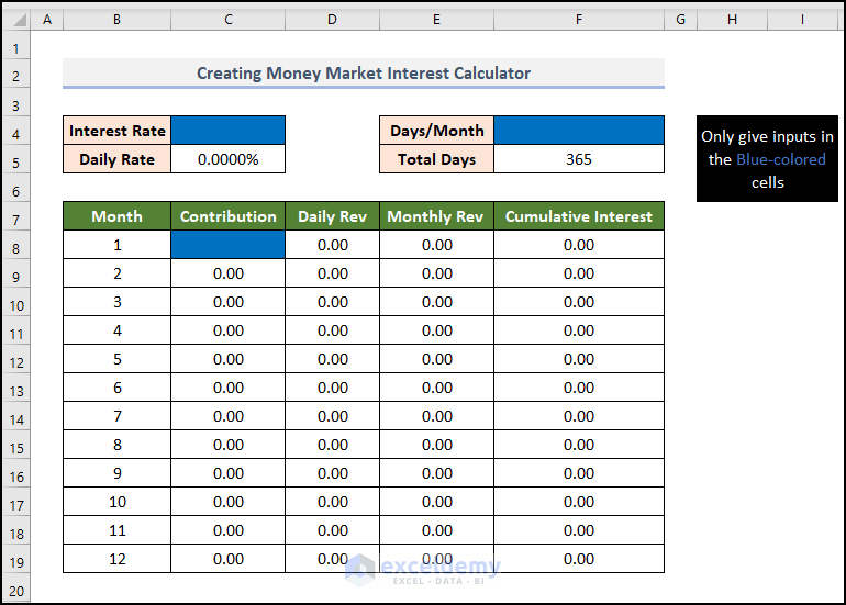
Free Template: Ready to Use

In the workbook below, we have added an extra sheet concluding with a free Money Market Interest Calculator template for your use. Change or edit it according to your needs. Just fill in the blue-colored cells, and the other calculations will be done automatically.