How to Use Cumulative Interest Formula in Excel (3 Easy Ways)

In finance, banking, or in business, it’s a quite common task to calculate cumulative or compound interest. We can calculate it in many ways. But Excel offers the easiest and time-saving ways to do it. So, today in this tutorial, we’ll learn 3 easy methods to use the cumulative interest formula in Excel with easy examples and vivid illustrations.

In this section, we will demonstrate three easy and effective ways to apply the cumulative interest formula in Excel.

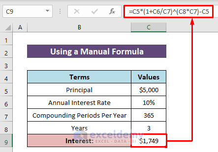
1. Using a Basic Mathematical Formula for Cumulative Interest

First, we’ll apply the basic mathematical formula in Excel to calculate compound interest. The function of the formula is simple, it will first calculate the final value over the periods and then will subtract the principal value from it to get the total cumulative interest.

The basic mathematical formula is:

• Cumulative/Compound Interest = P*(1+r/n)^t*n – P

Where,

• P is the principal.
• r is the annual interest rate.
• t is the time.
• n is the number of compounding.

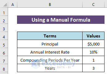
1.1 Yearly Compounding

Firstly, we’ll learn to apply the manual formula for yearly compounding, which means the compounded interest will be applied annually.

Let, a person take a loan of $5000 for 3 years at a 10% annual rate.

Steps:

• In Cell C9, insert the following formula:

• Then just hit the Enter button for the output.

As the compounding period per year is 1 here, so we skipped it in the formula.

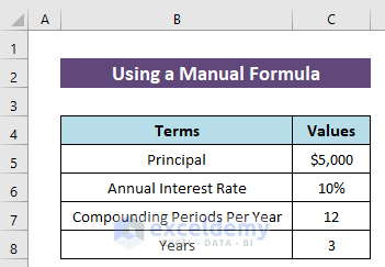
1.2 Monthly Compounding

For monthly compounding, the compounding period per year is 12. So, we’ll have to divide the annual rate by 12 and will have to multiply the number of years by 12 to get the total monthly periods. We’ll use the previous dataset to calculate the monthly cumulative interest.

Steps:

• Write the following formula in Cell C9–

• Next, press the Enter button to finish.

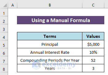
1.3 Weekly Compounding

To calculate weekly compounding interest, the compounding period per year is 52. So, we’ll have to divide the annual rate by 52, and to get the total weekly periods we’ll have to multiply the number of years by 52. Here also we’ll use the previous dataset to calculate the weekly cumulative interest.

Steps:

• Type the following formula in Cell C9–

• Later, hit the Enter button to get the compounded interest.

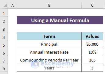
1.4 Daily Compounding

As one year is equal to 365 days, for daily compounding, we’ll divide the annual rate by 365, and to get the total daily periods, we’ll multiply the number of years by 365.

Steps:

• In Cell C9, insert the following formula:

• Finally, just press the Enter button for the output.

Read More: How to Calculate Daily Interest in Excel (2 Easy Ways)

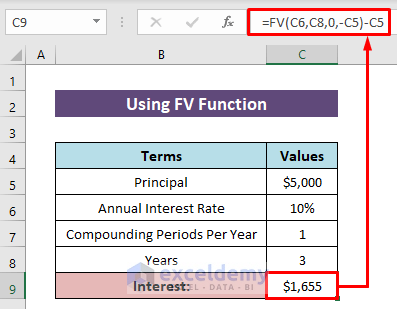
2. Using the FV Function to Calculate Cumulative Interest in Excel

Instead of using a manual formula, Excel has some functions that we can apply in a formula to calculate cumulative interest. In this method, we’ll apply the FV function to calculate the future value over a certain period and then will subtract the principal value to get the compound interest. We’ll apply the same dataset from the first method to get the cumulative interest for one year.

Steps:

• Apply the following formula in Cell C9–

• Then hit the Enter button to return the output.

Have a look, we got the same output as like the first section of the first method.

Read More: Simple Interest Formula in Excel (With 3 Practical Examples)

Similar Readings

• How to Calculate Accrued Interest on Fixed Deposit in Excel (3 Methods)
• Bank Interest Calculator in Excel Sheet – Download Free Template
• How to Find Interest Rate in Future Value Annuity (2 Examples)
• Create Post-Judgment Interest Calculator in Excel (With 2 Cases)
• Perform Carried Interest Calculation in Excel (with Easy Steps)

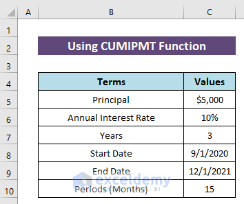
3. Using the CUMIPMT Function to Calculate Cumulative Interest Between Two Dates

The previous methods only return the cumulative interest for the whole period, they can’t calculate the interest for any range of specific periods within the whole period. But using the CUMIPMT function of Excel, we can calculate cumulative interest between two dates means the interest for any range of periods. Assuming, you have a loan of 60 months of the period then you can calculate the compound interest for the period from 5 to 30.

For this method, we modified the dataset. Let, a person has taken a loan of $5000 for 3 years/ 36 months at a 10% annual rate on 9/1/2020. Now we’ll find the interest between two dates- 9/1/2020 and 12/1/2021, the difference between the dates is 15 months of period. For the interest of these 15 months, we’ll use 1 for the start period and 15 for the end period in the formula.

Steps:

• In Cell C11, insert the following formula-

• Finally, press the Enter button to get the cumulative interest for the period.

This function returns the interest in a negative value, to avoid it, you can use a negative sign before the function.

Read More: How to Calculate Interest Between Two Dates Excel (2 Easy Ways)

Download Practice Workbook

You can download the free Excel workbook from here and practice independently.

Conclusion

That’s all for the article. I hope the procedures described above will be good enough to use the cumulative interest formula in Excel. Feel free to ask any question in the comment section and please give me feedback.

Related Articles

• How to Use Nominal Interest Rate Formula in Excel
• Nominal vs Effective Interest Rate in Excel (2 Practical Examples)
• Create Late Payment Interest Calculator in Excel and Download for Free
• How to Calculate Principal and Interest on a Loan in Excel
• How to Calculate Home Loan Interest in Excel (2 Easy Ways)
• Car Loan Calculator in Excel Sheet – Download Free Template