How to Calculate GPF Interest in Excel (with Easy Steps)

The article will show you how to calculate GPF (General Provident Fund) interest in Excel. Provident Fund is an account in which a certain percentage of the basic salary is deposited. After retirement or departure from the company, an employee gets this money. Employees can take a loan against this fund, as per some company rules. You can have a clear idea how to calculate GPF interest after reading this article.

What Is GPF Interest?

Government or non-government personnel can use the General Provident Fund (GPF) as an excellent savings tool. This is calculated through an interest rate which is known as GPF interest. Until the end of his or her employment, the employee may routinely contribute a portion of their pay. The company transfers the entire accumulated balance in the GPF account to the employee upon retirement.

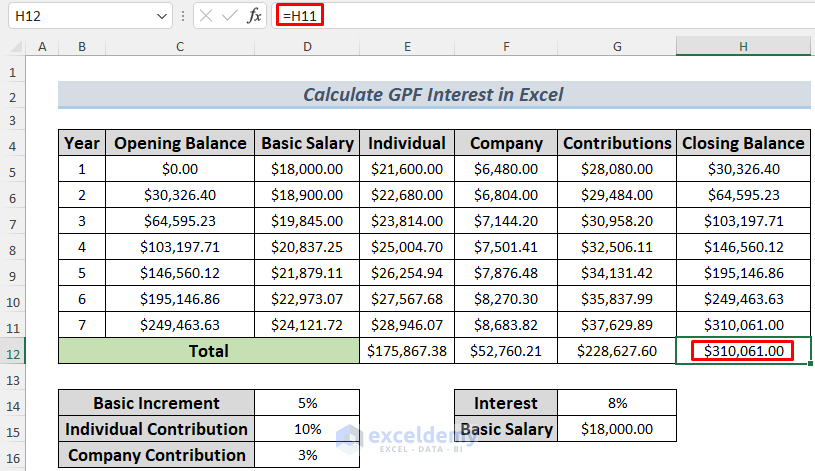
Steps to Calculate GPF Interest in Excel

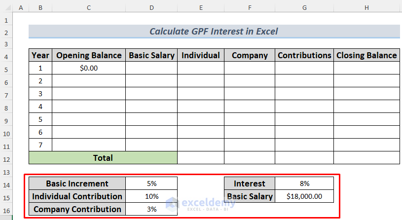
In the following picture, I’ll show you what a Provident Fund dataset looks like in Excel. The Provident Fund is calculated based on various parameters: Basic Salary, Employee and Company Contributions, Increment, etc. Here, we show the PF balance for 7 years.

Step-1: Inserting Primary Data

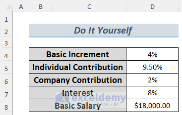
We determine the Provident Fund by using different variables. So we need to insert them first.

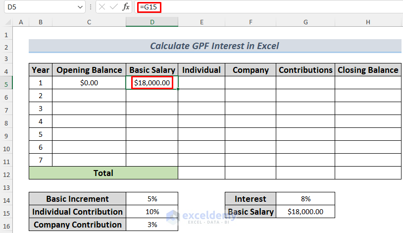
First, make some columns to store the variables and insert the primary data. We need the amount of Basic Salary, Interest Rate, Basic Increment, Individual and Company Contributions. Here I’m showing a general example of the General Provident Fund interest of an employee.

Step-2: Calculating Basic Salaries for 7 Years

After inserting the basic data for calculating GPF interest, we need to calculate the Basic Salaries for the next 7 years based on the yearly increment.

First, type the following formula in cell C5 and press ENTER. This formula will store the Basic Salary in C5.

=G15

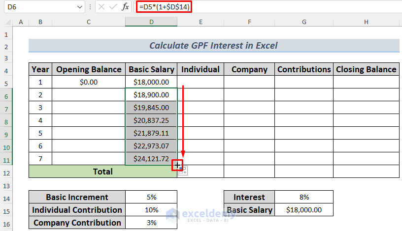
In order to calculate the Basic Salaries for the upcoming years, type the formula in cell D6 and press ENTER.

=D5*(1+$D$14)

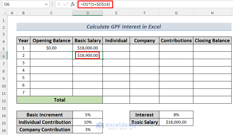
Next, use the Fill Handle to AutoFill the lower cells up to D11.

Step-3: Determining Individual and Company Contributions

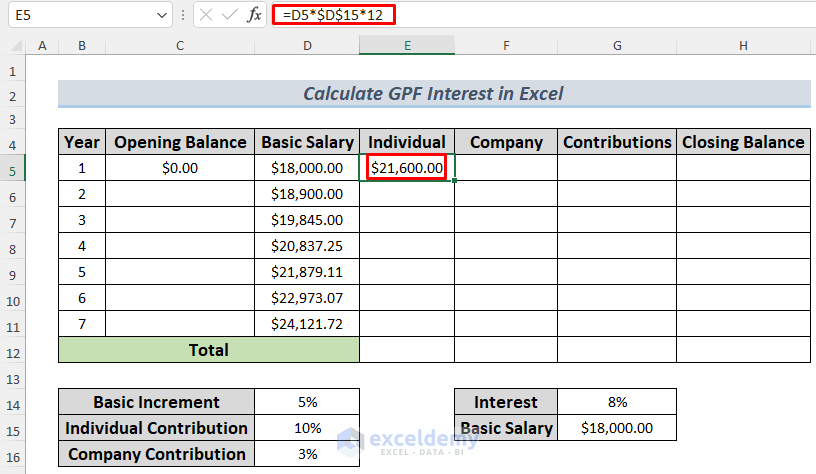
We also need to know the Individual and Company contributions. For that reason, we will have to apply some formulas.

First, use the following formula to calculate the Individual Contribution for the first year.

=D5*$D$15*12

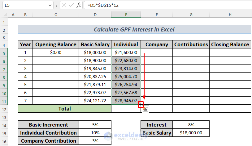
Next, drag the Fill Handle icon downwards to determine Individual Contributions for the upcoming years.

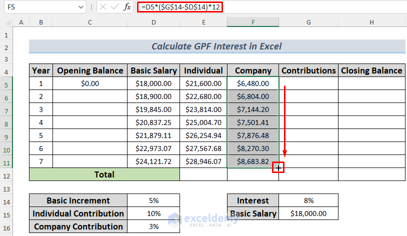
Similarly, type the following formula to calculate the Company Contributions.

=D5*($G$14-$D$14)*12

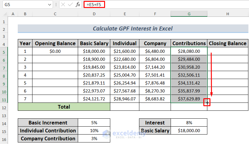
Next, we will simply store the total Contributions by using the following formula.

=E5+F5

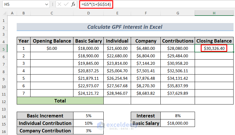
Step-4: Calculating Closing Balance

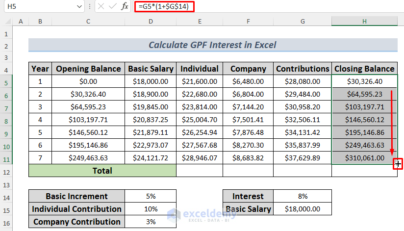
Finally, we will calculate the Closing Balance which is the total General Provident Fund interest after each year. Let’s follow the description below.

First, write down the formula below in cell H5. This will return the Closing Balance amount of the first year.

=G5*(1+$G$14)

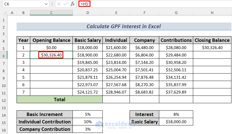
The Closing Balance of the first year is the second year’s Opening Balance. For this reason, we store this value in C66 using the formula below.

=H5

After that, use the Fill Handle to AutoFill the lower cells.

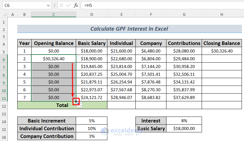
Thereafter, type the following formula to calculate the Closing Balance for the second year.

=(C6+G6)*(1+$G$14)

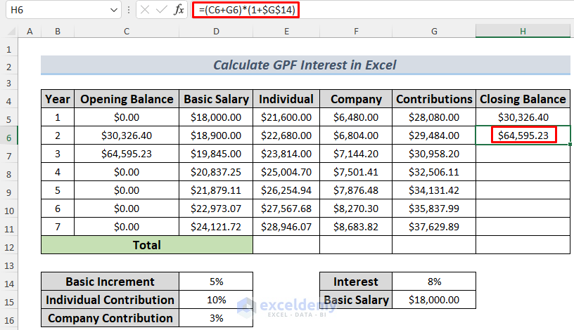
Finally, drag the Fill Icon downwards to H11 to AutoFill the lower cells. You can also notice that the Opening Balance column fills up automatically.

Step-5: Calculating the Gross Total

Finally, we will calculate the total amount of Individual and Company Contributions and the Closing Balances. If an employee retires or departs from the company after this period, the management should return him/her the total amount of the Closing Balance that we determine next in the dataset.

First, type the following formula in E12 to calculate total Individual Contribution.

=SUM(E5:E11)

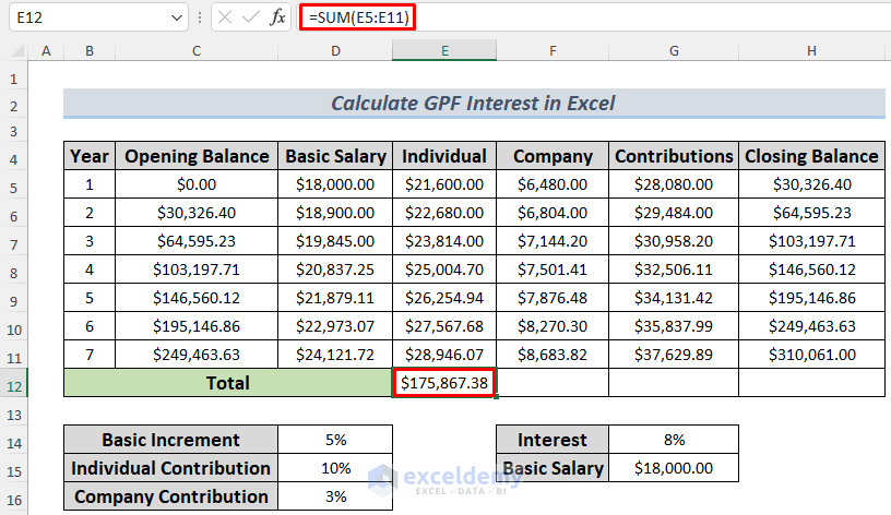
The formula uses the SUM function to return the total Individual Contributions.

Next, drag the Fill Handle icon to the right to calculate Company and Total Contributions.

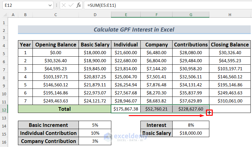
In the end, we simply store the final Closing Balance amount using the formula below. We finally calculate the GPF interest using Excel formulas.

=H11

Thus, you can calculate GPF interest in Excel.

Practice Section

Here, I’m giving you a new dataset so that you can practice these steps on your own.

Download Practice Workbook

Calculate GPF Interest.xlsx

Conclusion

Suffice to say, you will get a clear view of calculating GPF interest in Excel after reading this article. If you have any better suggestions or questions or feedback regarding this article, please share them in the comment box. This will help me enrich my upcoming articles.

<< Go Back to Calculate Interest In Excel | Excel for Finance | Learn Excel

Get FREE Advanced Excel Exercises with Solutions!