PPMT Function in Excel to Calculate Principal
The PPMT function calculates the principal of a financial product or service (e.g. total investments, loans, etc.) for a given period of time.
Purpose
To calculate the principal of a given investment.
Syntax
IPMT Function in Excel to Calculate Interest
The IPMT function calculates the interest portion of a financial product or service (e.g. investments, loans, etc.) for a given period of time.
Purpose
To calculate the interest of a given investment.
Syntax
Function Parameters
The parameters inside both of the functions are the same.
| Parameter | Required/ Optional | Description |
|---|---|---|
| rate | Required | The constant interest rate per period. |
| per | Required | The period for which the required value should be calculated. |
| nper | Required | The total number of payment periods for the given amount. |
| pv | Required | The present value or the total value for all types of payments. Must be entered as a negative number. If omitted, it is assumed to be zero (0). |
| [fv] | Optional | The future value, meaning the desired cash balance after the last payment. If omitted, it is assumed to be zero (0). |
| [type] | Optional | Indicates when payments are due with the number 0 or 1.
|
Calculate the Principal and Interest on a Loan in Excel
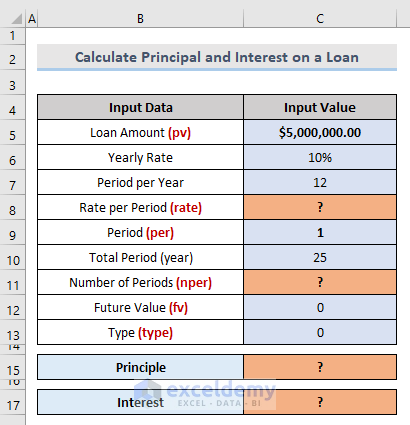
- Loan Amount -> $5,000,000.00 -> The loan amount. It must be entered as a negative value.
- Yearly Rate -> 10% -> 10% interest rate should be paid annually.
- Period per Year -> 12 -> There are 12 months in a year.
- Period -> 1 -> To get the result for the first month, the input is 1. This value is variable.
- Total Period(year) -> 25 -> The number of years allowed to pay off the total loan amount.
- Future Value -> 0 -> No required future value, so the [fv] input is 0.
- Type -> 0 -> To calculate a payment that is due at the end of the period, the input is 0.
In the above example, there are two parameters to find before calculating the principal and interest—rate and nper.
To calculate the Rate per Period (rate), divide the Yearly Rate (10% in this case) by the Period per Year (12).
rate = Yearly Rate/ Period per Year = Cell C6/ Cell C7 = 10%/12 = 0.83%
To calculate the Number of Periods (nper), multiply the Total Period (25) by the Period per Year (12).
nper = Total Period*Period per Year = Cell C10*Cell C7 = 25*12 = 300
All parameters are now available.
- rate = 83% -> Cell C8
- per = 1 -> Cell C9
- nper = 300 -> Cell C11
- pv = -$5,000,000.00 -> Cell C5
- [fv] = 0 -> Cell C12
- [type] = 0 -> Cell 13
- To calculate the principal, select the appropriate cell and enter the following formula:
=PPMT(C8,C9,C11,-C5,C12,C13)- Press Enter.
- To calculate interest, select the appropriate cell and enter the following formula.
=IPMT(C8,C9,C11,-C5,C12,C13)- Press Enter.
Things to Remember
- The period of interest is referred to as the parameter per. It must be a numeric value from 1 to the total number of periods (nper).
- The argument rate must be constant. For instance, if the annual interest rate is 7.5% for a 10-year loan, then calculate it as 7.5%/12.
- The argument pv has to be entered as a negative number.
Download Practice Workbook
You can download the free practice Excel workbook from here.
Related Articles
- How to Calculate Gold Loan Interest in Excel
- How to Calculate Credit Card Interest in Excel
- How to Calculate Home Loan Interest in Excel
- How to Calculate Accrued Interest on Fixed Deposit in Excel
- How to Calculate Accrued Interest on a Bond in Excel
- How to Calculate Accrued Interest on a Loan in Excel
<< Go Back to Excel for Finance | Learn Excel
Get FREE Advanced Excel Exercises with Solutions!
