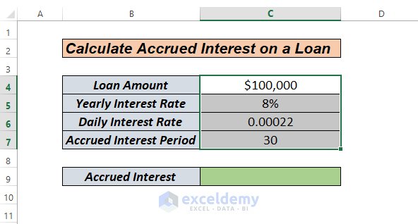
We will use a sample data set containing the Loan amount, Yearly Interest Rate, Daily Interest Rate, and Accrued Interest Period to Calculate Accrued Interest on a Loan.
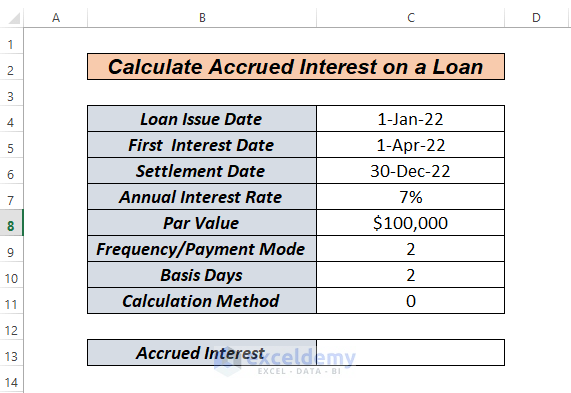
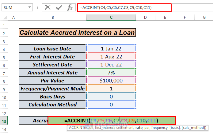
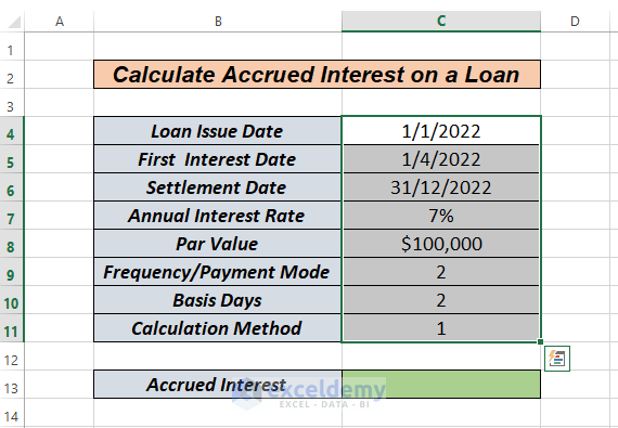
We will use also use the data set containing the Loan Issue Date, First Interest Date, Settlement Date, Annual Interest Rate, Par Value, Frequency or Payment Mode, Basis Days, and Calculation Method.
3 Simple Methods to Calculate Accrued Interest on a Loan in Excel
Method 1 – How to Calculate Accrued Interest on a Loan in Excel Manually
- Click on cell C6 and use the following formula.
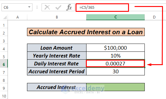
=C5/365
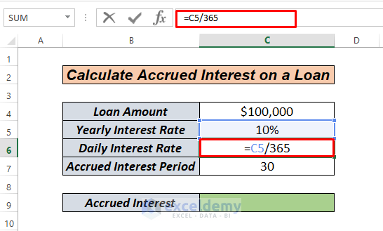
We are calculating the daily interest rate by simply dividing the yearly interest rate by the 365 number of days.
- Press the Enter key. We will get our daily interest rate as follows.
- Click on cell C9 and use the following formula.
=C4*C6*C7
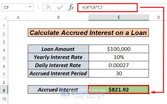
- Press the Enter key.
Read More: How to Calculate Accrued Interest on Fixed Deposit in Excel
Method 2 – How to Calculate Accrued Interest on a Loan in Excel Using the ACCRINT Function
If we look at sample dataset 2, we will see that this accrual interest method is different. In Excel, the function ACCRINT looks like the following.
=ACCRINT(issue, first_interest, settlement, rate, par, frequency, [basis], [calc_method])
First_interest: The date when the interest payment will first occur.
Settlement: The date when the loan will finish.
Rate: Annual or Yearly Interest rate.
Par: The loan amount.
Frequency: This is the annual number of loan payments. Annual payments will have a frequency of 1; semiannual payments will have a frequency of 2, and quarterly payments will have a frequency of 4.
Basis: This argument is optional. This is the type of day count used to calculate the interest on a certain loan or security. The base is set to 0 if the argument is omitted. Any of the following values can be used as the basis:
0 Or Omitted- US (NASD 30/360)
1- Actual/Actual
2- Actual/360
3- Actual/365
4-European 30/360
Calculation_method: It’s either 0 or 1 (calculates accrued interest from the first interest date to the settlement date). This argument is also optional.
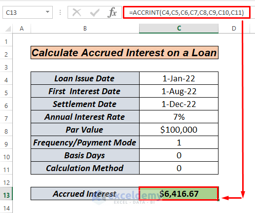
- Click on cell C13 and insert the following.
=ACCRINT(C4,C5,C6,C7,C8,C9,C10,C11)
- Press the Enter key.
Read More: How to Calculate Accrued Interest on a Bond in Excel
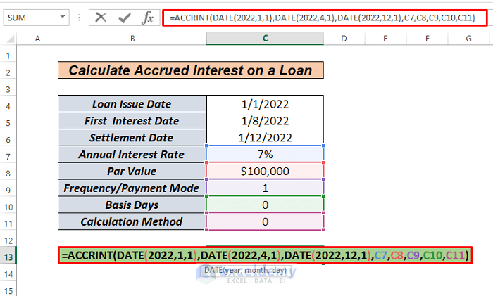
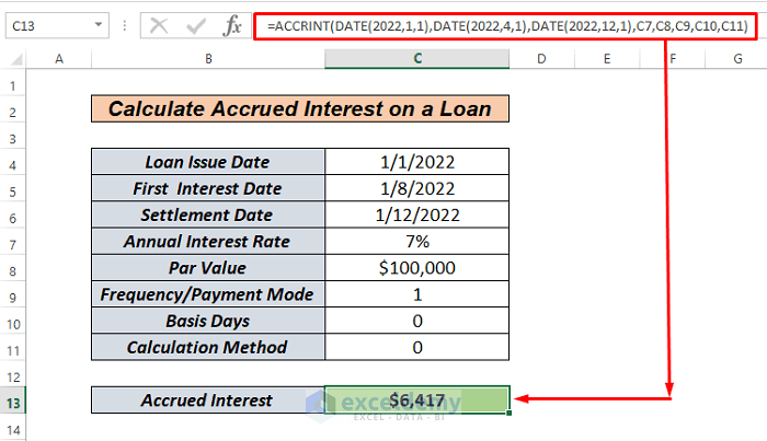
Method 3 – Calculate Accrued Interest on a Loan in Excel Using ACCRINT along with the Date Function
Our Issue Date, First Interest Date, and Settlement Date values are not formatted as Date.
- Click on cell C13 and enter the following formula.
=ACCRINT(DATE(2022,1,1),DATE(2022,4,1),DATE(2022,12,1),C7,C8,C9,C10,C11)
- Press the Enter key.
Read More: How to Calculate Interest on a Loan in Excel
Things to Remember
- The arguments for the first interest date and settlement date should be valid dates.
- You have to be aware of different date systems or date interpretation settings.
- For Basis, refer to the following table:
| Basis | Day Count Basis | Defined Year | Year Count |
|---|---|---|---|
| 0 | Or Omiited- US (NASD 30/360) | 360/30 | 12 |
| 1 | Actual/Actual | 366/30 | 12.20 |
| 2 | Actual/360 | 360/30 | 12 |
| 3 | Actual/365 | 365/30 | 12.1667 |
| 4 | European 30/360 | 360/30 | 12 |
Practice Section
We’ve attached a practice workbook to test these methods.
Download the Practice Workbook
Related Articles
- How to Calculate Credit Card Interest in Excel
- How to Calculate Principal and Interest on a Loan in Excel
- How to Calculate Home Loan Interest in Excel
- How to Calculate Gold Loan Interest in Excel
<< Go Back to Excel for Finance | Learn Excel
Get FREE Advanced Excel Exercises with Solutions!

Hope this works. Thank you.
Hello Barney,
You are most welcome. Hopefully it will work.
Please let us know if it worked or not!
Regards
ExcelDemy