Method 1 – Determining the Fixed Loan Repayment for Every Month of the Year
Let’s break down how to calculate interest on a loan in Excel using the PMT function.
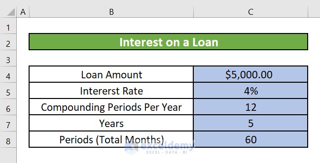
- Understanding the Scenario:
- Loan amount: $5,000
- Annual interest rate: 4% (expressed as a decimal, so 4% becomes 0.04)
- Loan term: 5 years (60 months)
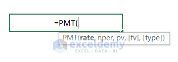
- Using the PMT Function: The PMT function calculates the fixed repayment for a loan based on constant payments and a constant interest rate. Here’s the syntax:
-
- rate : The interest rate per period (monthly in our case). Divide the annual rate by 12: C4/12.
- nper : The total number of payments (months): C7 (which is 60 in this scenario).
- pv : The principal amount (loan amount): C8 (which is $5,000).
- fv : The future value or a cash balance you want to attain after the last payment is made. If we do not insert a value for fv, it will be assumed as 0. For example, in the context of a loan, the future value would typically be 0 (since you aim to pay off the entire loan).
- type : The number 0 or 1. It indicates the time when the payments are due. If “type” is 0 (or omitted), payments are due at the end of each period (e.g., end of the month). If “type” is 1, payments are due at the beginning of each period (e.g., beginning of the month).
- Calculating the Monthly Repayment:
- In cell C10, enter the following formula:
=PMT(C4/12, C7, C8)
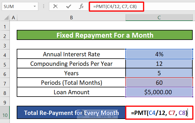
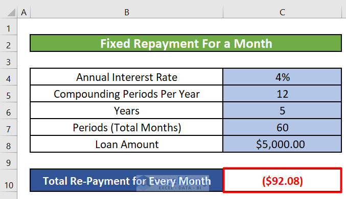
- When you press ENTER after entering the PMT formula in Excel, you’ll obtain the fixed monthly repayment amount. This amount remains consistent for every month and includes both the portion of the principal (capital) and the interest amount due in the first month.
- Calculating the Fixed Repayment for Every Year:
- In cell C10, enter the following formula:
=PMT(F4, F6, F8)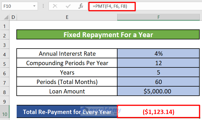
-
- This will give you the fixed annual repayment amount for the loan.
Remember to adjust the cell references according to your specific Excel sheet.
Read More: How to Calculate Principal and Interest on a Loan in Excel
Method 2 – Calculating the Interest Payment on a Loan for a Specific Month or Year
When you have a loan, the monthly or yearly repayment amounts remain the same throughout the loan term. However, the proportion of interest and capital you repay each period changes over time. Initially, you pay mostly interest and a small amount of capital, but by the end of the loan term, you pay mostly capital and very little interest.
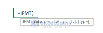
To calculate the interest payment for a specific month or year, you can use the IPMT function. Here’s how it works:
- Introduction to IPMT Function:
- Objective: The IPMT function calculates the interest payment for a given period (such as a specific month or year).
- Syntax:
-
- Return Parameter: The interest payment is based on periodic, constant payments and a fixed interest rate.
- Step-by-Step Calculation:
- Step 1: Select a cell (let’s say C10) and enter the following formula:
=IPMT(C4/12, 1, C7, C8)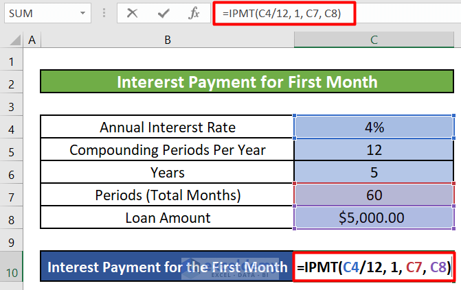
-
-
- Formula Breakdown:
- C4 (Rate): Annual Interest Rate (e.g., 4%)
- Since we’re calculating interest for a month, divide the annual rate by 12 (number of months in a year).
- 1 (Pr): The period for which you want to find the interest (e.g., 1 for the first month).
- C7 (Nper): Total number of payments (e.g., 60 for a 5-year loan).
- C8 (Pv): Total loan amount or Principal (e.g., $5,000).
- C4 (Rate): Annual Interest Rate (e.g., 4%)
- Formula Breakdown:
-
-
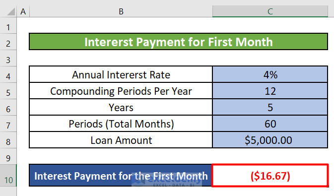
- Step 2: Press ENTER to get the interest amount for the first month.
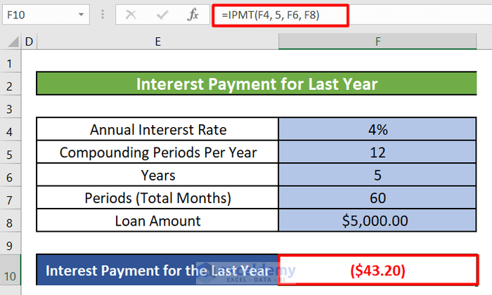
- Calculating Interest Payments for a Specific Year:
- To calculate the interest amount for the last year, enter the following formula:
=IPMT(F4, 5, F6, F8)
-
-
- Here:
- F4 represents the annual interest rate.
- 5 corresponds to the fifth year.
- F6 is the total number of payments.
- F8 is the principal amount.
- Here:
-
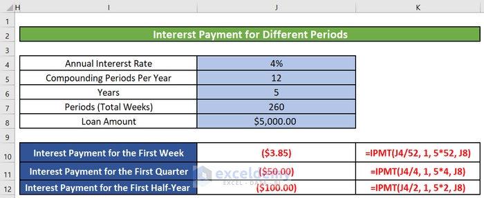
Calculating Interest Payments for Different Time Intervals:
We can also calculate the weekly, quarterly, and semi-annual interest payments using IPMT.
- Weekly Interest Payment:
- To calculate the weekly interest payment, adjust the formula as follows:
=IPMT(C4/52, 1, C7*52, C8)
-
-
- Here:
- C4/52 represents the weekly interest rate (annual rate divided by 52 weeks).
- 1 is the period (first week).
- C7*52 is the total number of payments (60 months converted to weeks).
- C8 is the principal amount.
- Here:
-
- Quarterly Interest Payment:
- For quarterly interest payments, enter this formula:
=IPMT(C4/4, 1, C7/3, C8)
-
-
- Here:
- C4/4 is the quarterly interest rate (annual rate divided by 4 quarters).
- 1 denotes the first quarter.
- C7/3 represents the total number of payments (60 months divided by 3 months per quarter).
- C8 is the principal.
- Here:
-
- Semi-Annual Interest Payment:
- To calculate semi-annual interest payments, enter:
=IPMT(C4/2, 1, C7/6, C8)
-
-
- Here:
- C4/2 corresponds to the semi-annual interest rate (annual rate divided by 2).
- 1 indicates the first semi-annual period.
- C7/6 is the total number of payments (60 months divided by 6 months per semi-annual period).
- C8 is the principal amount.
- Here:
-
Feel free to apply these formulas based on your desired time intervals to determine interest payments for your loan!
Method 3 – Computing Capital Payment for a Certain Interest Rate on a Loan
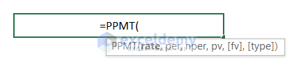
Let’s dive into the PPMT function in Excel. The PPMT function helps you determine the principal payment for a given period based on periodic, constant payments and a fixed interest rate. Here’s how it works:
- Syntax:
-
- rate : The interest rate per period.
- per : Specifies the payment period (must be in the range 1 to nper).
- nper : The total number of payment periods in an annuity.
- pv : The present value — the total amount that a series of future payments is worth now.
- [fv] (optional): The future value, or a cash balance you want to attain after the last payment is made. If omitted, it is assumed to be 0 (zero).
- type (optional): Indicates when payments are due (0 or 1). Set to 0 for payments at the end of the period or 1 for payments at the beginning of the period.
- Example: Let’s say we have the following data:
- Annual interest rate: 4%
- Number of years for the loan: 5
- Amount of loan: $5,000
- Applying the Formula: In cell C10, enter the following formula:
=PPMT(C4/12, 1, C7, C8)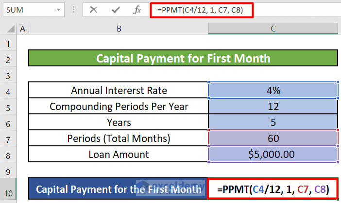
-
- C4/12 : This calculates the monthly interest rate by dividing the annual interest rate (C4) by 12.
- 1 : Since we’re interested in the first month, we set the period (per) to 1.
- C7 : This represents the total number of payments (60 in your case).
- C8 : The principal amount (total loan amount).
- Result: After pressing ENTER, you’ll get the capital amount to pay in the first month.
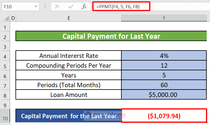
Additionally, if you want to calculate capital payments for a specific year (e.g., the last year), you can adjust the formula accordingly.
=PPMT(F4, 5, F6, F8)- F4 : Annual interest rate (no need to divide by 12 since we’re calculating for a year).
- 5 : The period (year) for which you want to find the capital payment (e.g., the 5th year).
- F6 : Total number of payments (5 years in your case).
- F8 : Principal amount.
Note: The sum of interest payment and capital payment will be equal to the fixed repayment amount that we calculated in the first method.

- Interest Payment for the First Month:
- You’ve calculated the interest payment for the first month using the IPMT function. The result is $16.67.
- The IPMT function helps determine the interest portion of a payment based on a fixed interest rate, total number of payments, and the present value (loan amount).
- Capital Payment for the First Month:
- You’ve calculated the capital payment for the first month using the PPMT function. The result is $75.42.
- The PPMT function calculates the principal payment for a specific period based on constant payments, a fixed interest rate, and the total number of payments.
- Total Payment for the First Month:
- By adding the interest payment and capital payment, we get the total repayment for the first month: $16.67 + $75.42 = $92.09.
- This matches the total repayment amount calculated using the PMT function in the first method.
- Consistency Across Identical Periods:
- The total amount to repay remains the same for every identical period (e.g., every month).
- However, the interest amount and capital amount will vary from period to period.
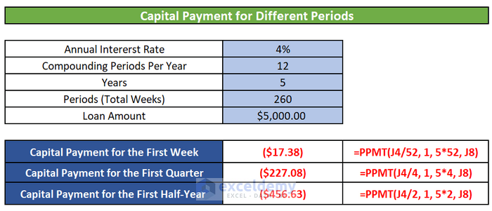
- Exploring Other Payment Frequencies:
- We can also calculate weekly, quarterly, and semi-annual capital payments using the PPMT function.
- Feel free to adjust the formula parameters to explore different payment frequencies based on your specific loan scenarios.
Remember to adapt these formulas according to your loan terms and payment schedules!
Method 4 – Calculating Cumulative Loan Interest for a Specific Month or Year in Excel
- Introduction to CUMIPMT Function:
- The CUMIPMT function calculates the cumulative interest paid on a loan between specified start and end periods.
- Its syntax is as follows:
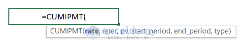
=CUMIPMT(rate, nper, pv, start_period, end_period, [type])
- Argument Explanation:
- rate : Annual interest rate (expressed as a decimal).
- nper : Total number of payments (e.g., 60 for a 5-year loan with monthly payments).
- pv : Total loan amount (principal).
- start_period : Starting period for cumulative interest calculation (e.g., 1 for the first month).
- end_period : Ending period for cumulative interest calculation (e.g., 60 for the last month).
- [type] : Payment type (0 for payment at the end of the period).
- Step-by-Step Calculation:
- Let’s assume we have a loan with the following details:
- Annual interest rate: 4%
- Total loan amount: $5,000
- Total number of payments: 60 (5 years with monthly payments)
- Let’s assume we have a loan with the following details:
-
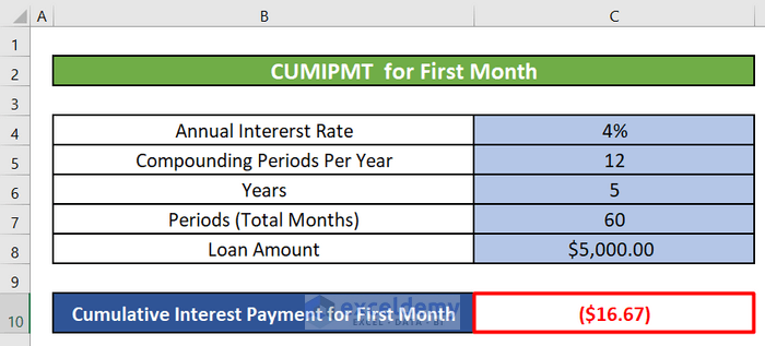
- To calculate cumulative interest for the first month (starting period = 1):
- Enter the following formula in cell C10:
- To calculate cumulative interest for the first month (starting period = 1):
=CUMIPMT(C4/12, C7, C8, 1, 1, 0)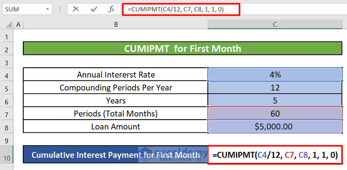
-
- C4/12 : This calculates the monthly interest rate by dividing the annual interest rate (C4) by 12.
- C7 : This represents the total number of payments (60 in your case).
- C8 : The principal amount (total loan amount).
- 1 : The start period and the end period. Since we’re interested in the first month, we set the start and end period (per) to 1.
- 0 : The number 0 or 1. It indicates the time when the payments are due. If “type” is 0 (or omitted), payments are due at the end of each period (e.g., end of the month). If “type” is 1, payments are due at the beginning of each period (e.g., beginning of the month).
-
-
- Press ENTER to get the cumulative interest amount for the first month.
-
-
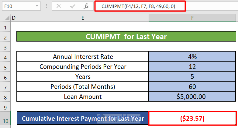
- To calculate cumulative interest for the last year (starting period = 49, ending period = 60):
- Enter the formula:
- To calculate cumulative interest for the last year (starting period = 49, ending period = 60):
=CUMIPMT(F4/12, F7, F8, 49,60, 0)-
-
- The starting period is 49 (after the 4th year), and the ending period is 60 (end of the 5th year).
-
- Fixed Annual Repayment Amount:
- Refer to the image below for the fixed annual repayment amount.
Read More: How to Calculate Accrued Interest on a Bond in Excel
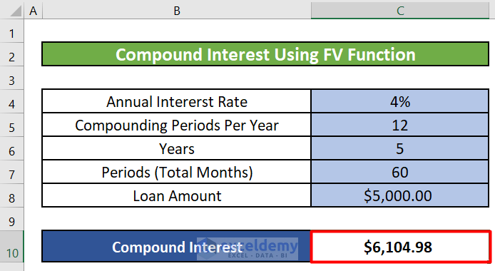
Method 5 – Using Excel FV Function to Calculate Compound Interest on a Loan
- Introduction to FV Function:
- The FV function in Excel calculates the future value of an investment based on a constant interest rate. You can use it for either periodic, constant payments or a single lump-sum payment.
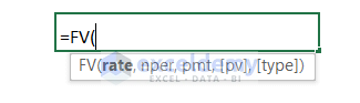
- Syntax of FV Function:
- The syntax for the FV function is as follows:
FV(rate,nper,pmt,[pv],[type])
-
-
- rate : The annual interest rate (expressed as a decimal).
- nper : The total number of payment periods (e.g., months or years).
- pmt : The payment made each period (can be zero if there are no regular payments).
- [pv] : The present value (initial investment or loan amount).
- [type] : Optional argument (0 or 1) indicating whether payments are due at the beginning or end of the period (0 for end, 1 for beginning).
-
- Step-by-Step Calculation:
- Let’s assume we have the following values:
- Annual interest rate (C4): 4% (expressed as 0.04)
- Total number of payments (C7): 60 (for a 5-year loan)
- Payment made each period (PMT): 0 (since we’re calculating compound interest)
- Present value (PV): -C8 (the loan amount, negative because it’s an outgoing payment)
- Let’s assume we have the following values:
- Formula for Compound Interest (First Month):
- In cell C10, enter the following formula:
=FV(C4/12, C7, 0, -C8)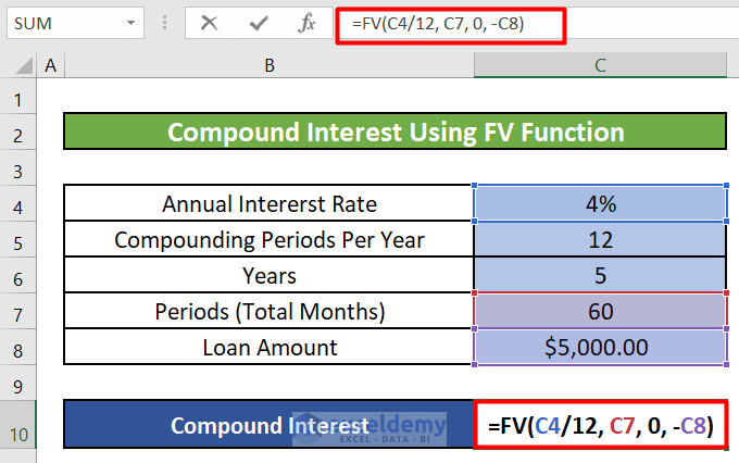
-
-
- C4/12 : Converts the annual interest rate to a monthly rate (since we’re calculating monthly).
- C7 : The total number of payments (60 months).
- 0 : No regular payments (since we’re calculating interest only).
- -C8 : The initial loan amount (negative sign because it’s an outgoing payment).
-
- Result:
- After entering the formula and pressing ENTER, you’ll get the compound interest for the first month.
Things to Remember
- The type argument in these functions is usually optional. It can take the values 0 or 1, indicating when payments are due.
- If the type argument is omitted, it is assumed to be 0 (payments due at the end of the period).
- Set the type argument to 0 if payments are due at the end of the period.
- Set type argument to 1 if payments are due at the beginning of the period.
Download Practice Workbook
You can download the practice workbook from here:
Related Articles
- How to Calculate Credit Card Interest in Excel
- How to Calculate Home Loan Interest in Excel
- How to Calculate Accrued Interest on Fixed Deposit in Excel
- How to Calculate Gold Loan Interest in Excel
- How to Calculate Accrued Interest on a Loan in Excel
<< Go Back to Excel for Finance | Learn Excel
Get FREE Advanced Excel Exercises with Solutions!

I LIKE TO USED THIS APP PLESED
Hello, OPIYO DENIS OCAYA! You can download our practice workbook and use it as a calculator which is quite similar to using an app instead!
Hi, I want to calculate how much money is paid to the bank for a loan in total, so I used CUMIPMT formula, but it shows a different number than simply PMT*nper, why is that?
And can I get to PMT*nper with a single formula?
Greetings Tom,
You are right. You can calculate the Total Paid or Payable Amount of a loan using PMT*nper or Cumulative Interest + Loan Amount. And the amount will be the same.
Make sure you enter the Start_period (i.e., minimum 1) and End_period (i.e., within the Total Periods (60)) correctly.
Regards,
Md. Maruf Islam (Exceldemy Team)