How to Calculate the Interest Between Two Dates in Excel (3 Ways)

Method 1 – Using the IPMT Function

Steps:

Enter the following formula in cell C12:

=IPMT(C5/12,1,C6*C7,C4)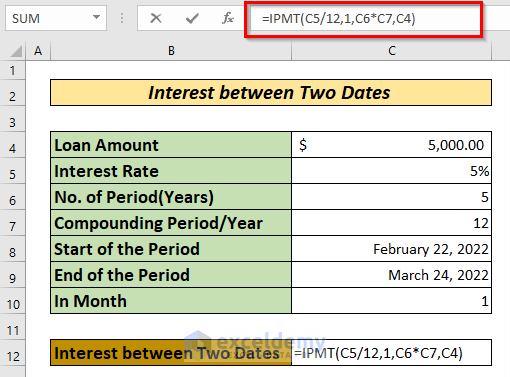

Formula Breakdown

Rate>>C5/12>> Converts annual interest rate to monthly interest rate.
Per>> 1>> We want to calculate the interest rate for 1 month.
Nper>>C6*C7>> Gives the total number of repayments. Here we have 5 years * 12 months/year= 60 repayments.
Pv>> C4>> Gives the principal amount of the loan.
IPMT(C5/12,1,C6*C7,C4)>> Gives the interest payment for the given period.

Press the ENTER key to find the interest between two dates in cell C12.

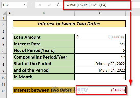
The minus sign before the amount of $18.75 denotes the cash outflow.

Note

The IPMT function does not consider the start and end dates. To consider the start and end dates, see the below methods.

Method 2 – Using Simple Interest

Stages:

Enter the following formula into cell C10:

=C4*(C8-C7)*(C5/365)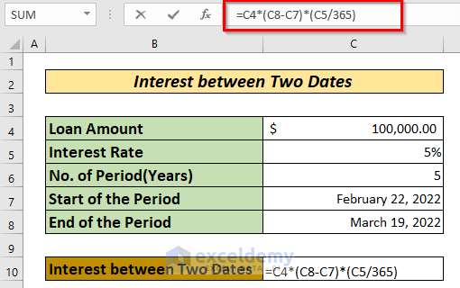

Formula Breakdown

C4>> Gives the principal amount.
C8-C7>> Gives the number of days between March 19, 2022 and February 22, 2022.
Output is>> 25 days
C5/365>> Gives the daily interest rate.
C4*(C8-C7)*(C5/365) >> Gives the product of the three i.e., the interest.

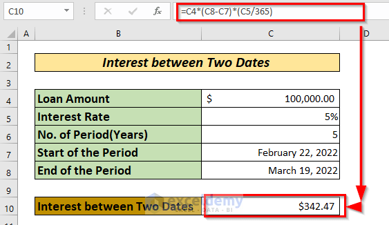
Press ENTER to find the interest in cell C10.

Method 3 – Using VBA Function

Steps:

Go to the Developer tab >> click Visual Basic.

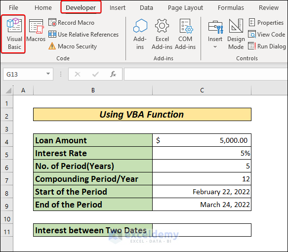
In the Visual Basic window, click on Insert >> Module >> enter the below VBA code. Close the window.

Function CalculateInterest(Principal As Double, AnnualInterestRate As Double, _
LoanTermInYears As Integer, CompoundingPeriodsPerYear As Integer, _
StartDate As Date, EndDate As Date) As Double
Dim MonthlyInterestRate As Double
Dim TotalPeriods As Integer
Dim Interest As Double
MonthlyInterestRate = AnnualInterestRate / CompoundingPeriodsPerYear
TotalPeriods = LoanTermInYears * CompoundingPeriodsPerYear
Interest = -Principal * WorksheetFunction.IPmt(MonthlyInterestRate, _
DateDiff("m", StartDate, EndDate) + 1, TotalPeriods, 1, 0)
CalculateInterest = Interest
End Function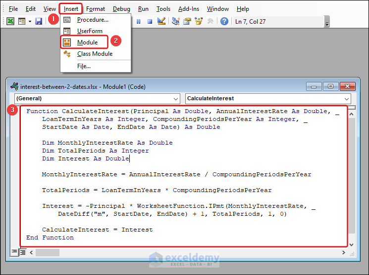

Enter the custom CalculateInterest function below in cell C11 >> press Enter.

=CalculateInterest(C4,C5,C6,C7,C8,C9)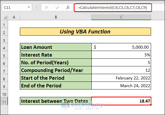

We get 18.47 as the interest between the dates in C8 and C9.

Practice Section

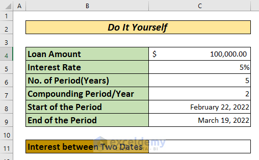
Below is a practice section so you can practice the methods.

Download the Practice Workbook

interest-between-2-dates.xlsm

<< Go Back to Excel for Finance | Learn Excel

Get FREE Advanced Excel Exercises with Solutions!

Function CalculateInterest(Principal As Double, AnnualInterestRate As Double, _ LoanTermInYears As Integer, CompoundingPeriodsPerYear As Integer, _ StartDate As Date, EndDate As Date) As Double

Function CalculateInterest(Principal As Double, AnnualInterestRate As Double, _ LoanTermInYears As Integer, CompoundingPeriodsPerYear As Integer, _ StartDate As Date, EndDate As Date) As Double Dim MonthlyInterestRate As Double Dim TotalPeriods As Integer Dim Interest As Double MonthlyInterestRate = AnnualInterestRate / CompoundingPeriodsPerYear TotalPeriods = LoanTermInYears * CompoundingPeriodsPerYear Interest = -Principal * WorksheetFunction.IPmt(MonthlyInterestRate, _ DateDiff("m", StartDate, EndDate) + 1, TotalPeriods, 1, 0) CalculateInterest = Interest End Function

2 Comments

Misled Reader Sep 9, 2023 at 3:53 AM

Unfortunately I’m pretty sure your first example is incorrect. No where in the formula does it use either the beginning or ending dates (cells C8 & C9). You can see this by there lack of inclusion in the formula. Or, you can recreate this simple example and change the ending date do 12/31/2060 for example and the result is the same. All you’ve calculated is the interest payable in the 1st period of a 5 year note represented by the hardcoded “1” used in the “PER” section of the formula.
- Reply
  Yousuf Khan Sep 11, 2023 at 12:46 PM
  Hello MISLED READER,
  
  Thank you for reading our article and your feedback. You have specified an incorrect use of the IPMT function that does not consider the start and end dates. And, you are correct about the fact that the method calculates the interest payable in the 1st period of a 5 year note represented by the hardcoded “1” used in the “PER” section of the formula. The IPMT function returns interest rates based on periods and not specific calendar dates. Thank you for pointing out the article gap to us. We will fix the issue with correct information. For now, we will show you another method here.
  
  You can use the other Excel basic formula to calculate the interest between two dates. Or, enter a custom VBA function as described below.
  
  This function will take the loan details, including start and end dates, as input arguments and return the interest amount.
  Here is the syntax and arguments of the CalculateInterest function I have created:
```
Function CalculateInterest(Principal As Double, AnnualInterestRate As Double, _
    LoanTermInYears As Integer, CompoundingPeriodsPerYear As Integer, _
    StartDate As Date, EndDate As Date) As Double
```
  Here are the steps to implement the function:
  
  1. Save the below VBA code to a Module.
```
Function CalculateInterest(Principal As Double, AnnualInterestRate As Double, _
    LoanTermInYears As Integer, CompoundingPeriodsPerYear As Integer, _
    StartDate As Date, EndDate As Date) As Double

    Dim MonthlyInterestRate As Double
    Dim TotalPeriods As Integer
    Dim Interest As Double
    
    MonthlyInterestRate = AnnualInterestRate / CompoundingPeriodsPerYear
    
    TotalPeriods = LoanTermInYears * CompoundingPeriodsPerYear
    
    Interest = -Principal * WorksheetFunction.IPmt(MonthlyInterestRate, _
        DateDiff("m", StartDate, EndDate) + 1, TotalPeriods, 1, 0)
    
    CalculateInterest = Interest
End Function
```
  2. Now, enter the VBA function in cell C11 >> press Enter key to get the interest.
  
  This formula calculates the interest between February 22, 2022, and March 24, 2022, based on the provided loan details.
  
  Feel free to let us know your future queries and suggestions as we always appreciate them. Thank you.
  
  Regards,
  Yousuf Shovon