How to Create FD Interest Calculator in Excel (with Easy Steps)

Download Practice Workbook

Download this practice workbook to exercise while you are reading this article.

FD Interest Calculator.xlsx

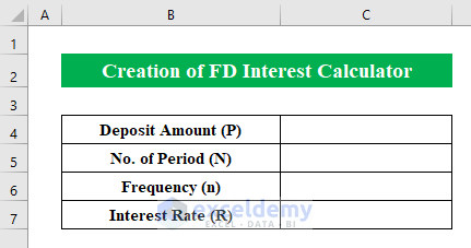
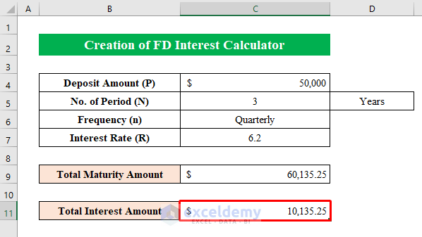
Step 1: Create a Dataset with Proper Information

First, create a dataset with some information to determine the fixed deposit interest and total amount.

As an exampel, this calculator will have “Deposit amount”, “No. of Period”, “Frequency”, and “Interest Rate”. These values will determine the interest amount.

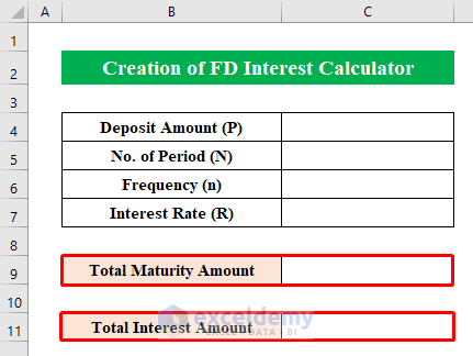
Create two cells with “Total Maturity Amount” and “Total Interest Amount” to collect the total amount.

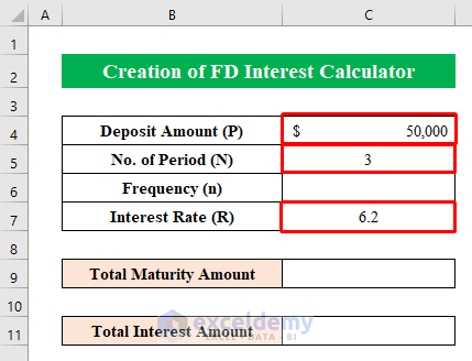
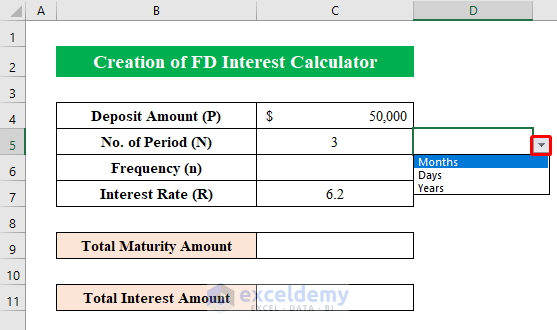
For an example of how the values will be filled, consider a “Deposit Amount” of $50,000, “No. of Period” is 3 years and an “Interest Rate” of 6.2%.

Step 2: Categorize Deposit Frequency

Before you can calculate the interest, you need to determine the deposit frequency and its duration.

As the fixed deposit can be calculated over days, months, and years, you can use a drop-down list to allow the user to pick the corresponding option and avoid confusion.

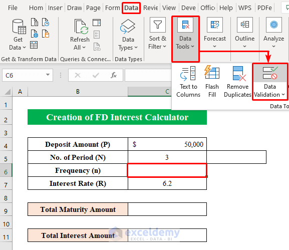
Start with the cell next to the period number (D5).
Choose the “Data Validation” option from the “Data” toolbar on the top.

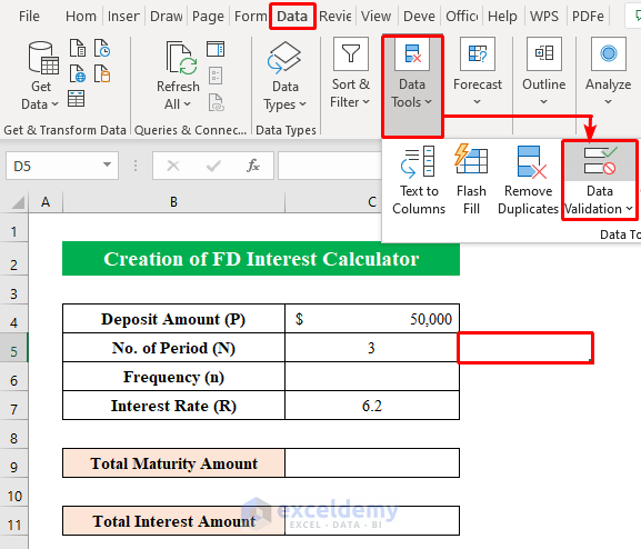
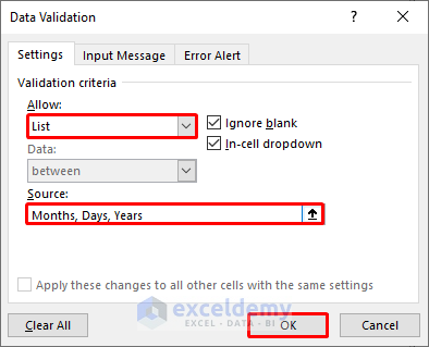
A new dialog box will pop up named “Data Validation.”
From the box, choose “List” from the drop-down list and type “Months, Days, Years” in the “Source” section. Each term should be separated by a comma. Spaces between terms are ignored.
To finish, click OK.

When you get back to the worksheet, you can see that the cell will contain a drop-down with the listed options.

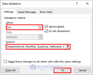
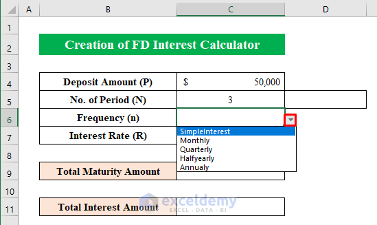
Make a drop-down list for the cell C6 to allow for a more customizable input for interest frequency calibration in the same way.

For the allowed values, type “SimpleInterest, Monthly, Quarterly, Halfyearly, Annually” in the source section. Make sure to remember the exact spelling you used for compound words.
Hit OK to confirm.

You can test the C6 drop-down or change the terms to be more human-readable.

Step 3: Apply Formula to Calculate FD Interest

With the drop-downs and list terms ready, you can create the bulk of the calculator. This will be a single, quite large formula. If you’ve used the exact terms for the list units above, copy the following formula directly to cell C9:

=IF(C6="SimpleInterest",(C4*(1+((C7*5)/((IF(D5="years",1,IF(D5="months",12,IF(D5="days",365))))*100)))),IF(C4="Annually",(C4*(1+(C7/100))^(C5*(1/(IF(D5="years",1,IF(D5="months",12,IF(D5="days",365))))))),IF(C6="Halfyearly",(C4*(1+(C7/(100*2)))^(C5*(2/(IF(D5="years",1,IF(D5="months",12,IF(D5="days",365))))))),IF(C6="Quarterly",(C4*(1+(C7/(100*4)))^(C5*(4/(IF(D5="years",1,IF(D5="months",12,IF(D5="days",365))))))),IF(C6="Monthly",(C4*(1+(C7/(100*12)))^(C5*(12/(IF(D5="years",1,IF(D5="months",12,IF(D5="days",365))))))))))))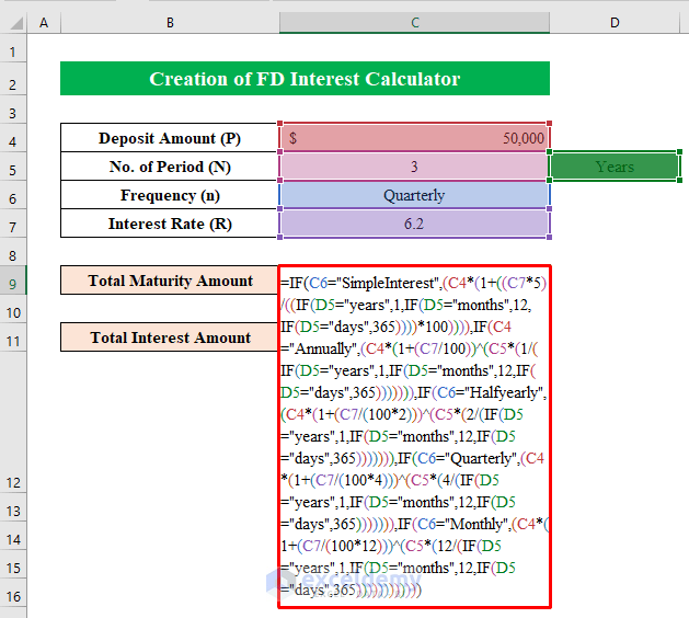

Formula Breakdown:

This is essentially a nested IF formula that returns a specific interest calculation based on the value find in C6.
=IF(C6=”SimpleInterest”,(C4*(1+((C7*5)/((IF(D5=”years”,1,IF(D5=”months”,12,IF(D5=”days”,365))))*100))))) → Here, the IF function will display the calculated amount if the statement (C4*(1+((C7*5)/((IF(D5=”years”,1,IF(D5=”months”,12,IF(D5=”days”,365))))*100)) is true otherwise it will move to the next argument.
Similarly, the IF function will run the argument for “Annually, Halfyearly, Quarterly, Monthly” selections from the drop-down list in cell (C6) until it finds the proper selection. After matching the selection from the cell (C6), it will calculate the amount matching the criteria from this argument (IF(D5=”years”,1,IF(D5=”months”,12,IF(D5=”days”,365))))*100) which explains if the value in cell (D5) is in years it will multiply the cell (C5) value with 1. Otherwise, move to the next loop search for the proper selection, and display output according to it.

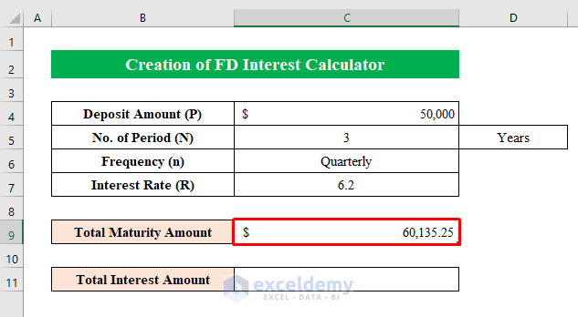
Hit ENTER to apply the formula and get the “Total Maturity Amount” based on the values you chose or put into the table.

The actual accrued interest (C11) is calculated by subtracting the “Total Maturity Amount” from the “Deposit amount” by using the simple formula:

=C9-C4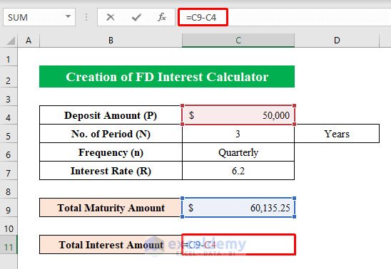

You can play around with different values.

Things to Remember

Don’t forget to put closing parenthesis at the end of the function. Otherwise, the formula won’t work.

Conclusion

This is a relatively simple and brute-force implementation of the interest calculator. If you need to introduce additional interest variables (such as different frequencies), you will need to modify the IF function accordingly. Alternatively, you can replace the nested IFs with SWITCH functions, which can make the formula more readable overall.