How to Create a Monthly Accrued Interest Calculator in Excel

The Accrued Interest is the payable or receivable interest on a loan or bond after a period of time.

Monthly Accrued Interest Calculator in Excel

Download the Excel Template

Download the Template.

Monthly Accrued Interest Calculator.xlsx

Accrued Interest

The formula to calculate the accrued interest is:

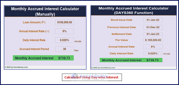
Accrued Interest = Loan Amount or Par Value ✖ ( Yearly Interest/365)✖ Period of Interest Accrued

Method 1 – Applying the Accrued Interest Formula

Provide Loan Amount, Annual Interest Rate, and Accrued Interest Period to find the accrued interest amount.

Accrued Interest = Loan Amount or Par Value ✖ ( Yearly Interest/365)✖ Period of Interest Accrued

Enter the formula into any cell.

=PRODUCT(C3,C7,C9)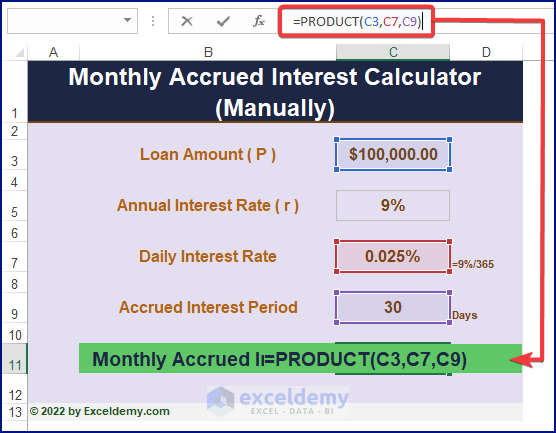

Accrued Interest Formula

Formula Breakdown

Loan Amount or Par Value = C3
Yearly Interest = C7
Period of Interest Accrued = C9

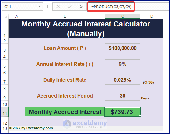
Press ENTER to find the monthly accrued interest on bonds or loans.

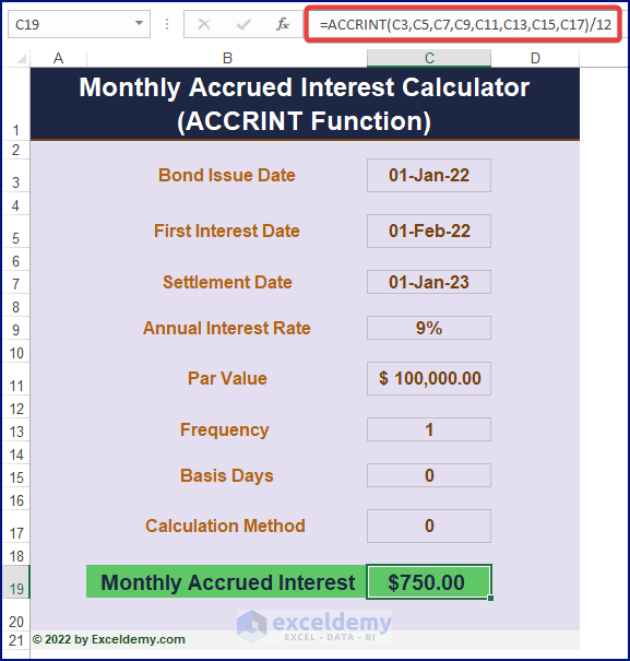
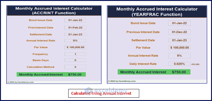
Method 2 – Using the ACCRINT Function

The syntax is:

=ACCRINT(issue, first_interest, settlement, rate, par, frequency, [basis], [calc_method])

The Arguments

Issue: The date when a loan or bond is issued.

First_interest: The date of the first interest payment.

Settlement: The end date of the loan.

Rate: Annual or Yearly Interest rate.

Par: The loan amount.

Frequency: The annual number of loan payments. 1 for Annual, 2 for Semi-annual, and 4 for Quarterly payments.

Basis: The basis is set to 0 if the argument is omitted. [Optional]

Calculation_method: It’s either 0 or 1 (calculates accrued interest from the First_interest date to the Settlement date). [Optional]

Use the formula in a blank cell.

=ACCRINT(C3,C5,C7,C9,C11,C13,C15,C17)/12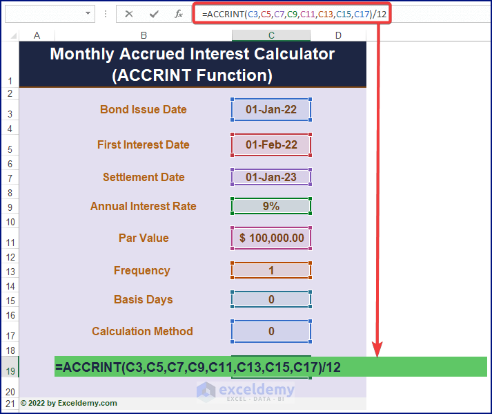

ACCRINT Function to be used as Monthly Accrued Interest Calculator in Excel

Press ENTER to display the accrued interest.

Method 3 – Counting Days Using the DAYS360 Function

The syntax is:

Days360(start_date,end_date,[method])

Multiplying the outcome by the Daily Interest Rate and Par Value will return the monthly accrued interest. Make sure the difference between the two dates is one (1) month.

Enter the formula to find the accrued interest.

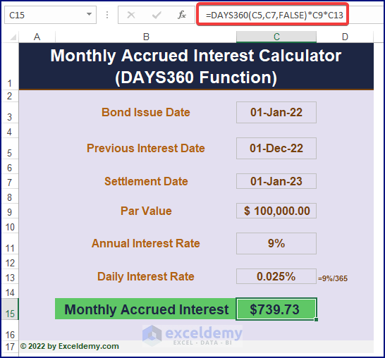
=DAYS360(C5,C7,FALSE)*C9*C13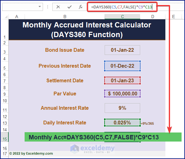

Press ENTER to display the amount.

Method 4 – Finding the Year Fraction using the YEARFRAC Function

The syntax of the function is:

YearFrac(start_date, end_date, [basis])

The returned value is multiplied by 365, Par Value, and Annual Rate to display the accrued interest. For the monthly accrued interest, the two dates must be one month apart.

Enter the below formula in a cell.

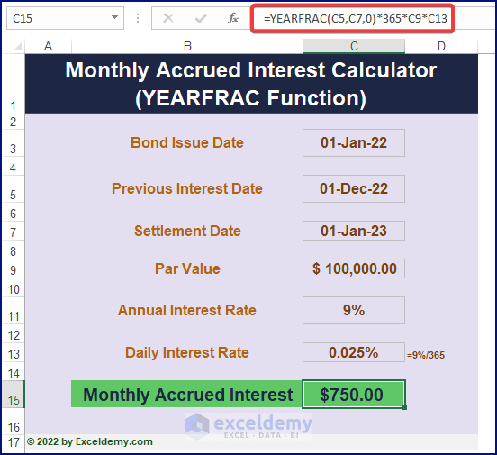
=YEARFRAC(C5,C7,0)*365*C9*C13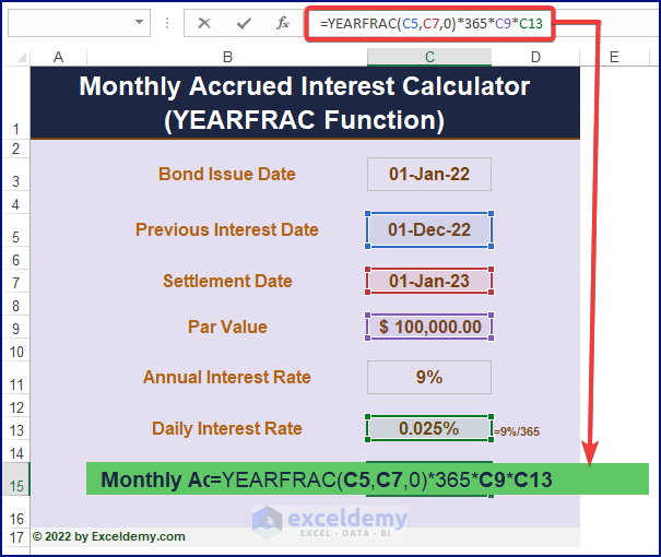

Press ENTER to display the accrued interest.

Cross-checking the Accrued Interest Value

Two different values are returned for the monthly accrued interest because two different approaches were used:

a. Daily Interest Rate

It takes the annual interest rate and divides it by 365. This result is multiplied by the Par Value, Daily Interest Rate and 30 (days in a month).

Monthly Accrued Interest Calculator in Excel-Daily Interest