How to Create GST Interest Calculator in Excel (with Useful Steps)

If you are looking for how to create a GST interest calculator in Excel, then you are in the right place. In Excel, while doing business calculations, we often need to calculate different financial statistics and obviously, we need to deal with GST. In this article, we’ll try to discuss how to create a GST interest calculator in Excel.

Download Practice Workbook

What Is GST?

GST stands for Goods and Service Tax. This is a value-added tax imposed on goods and services for domestic purposes. The final price of a good or service includes this tax. Although the consumer pays this tax, it is remitted to the government by the seller or the business.

Steps to Create GST Interest Calculator in Excel

Excel offers some easy steps to create a GST interest calculator. We just need to apply the arithmetic formulas correctly in the specific cells.

1. Creating Variable for GST Calculator

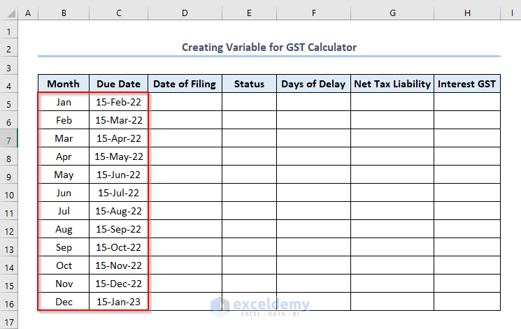
Firstly, we need to assign variable names for calculating GST interest and put them in the column headings. We have assigned the following variable names for our calculator.

• Month
• Due Date
• Date of Feeling
• Status
• Days of Delay
• Net Tax Liability
• Interest GST

Secondly, assign the Month and Due Date to file GST. We have created our calculator for the whole year( from January to December) and taken the Due Date 15th for every month. The variables added are like the picture below.

Read More: How to Create FD Interest Calculator in Excel (with Easy Steps)

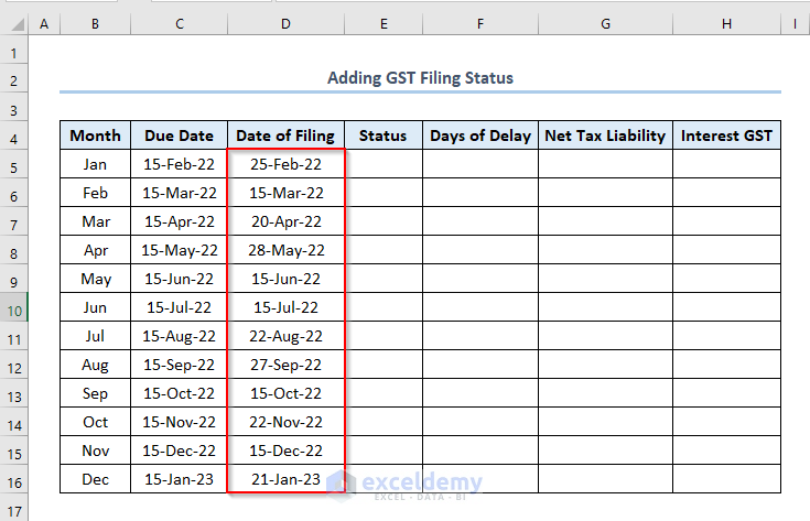
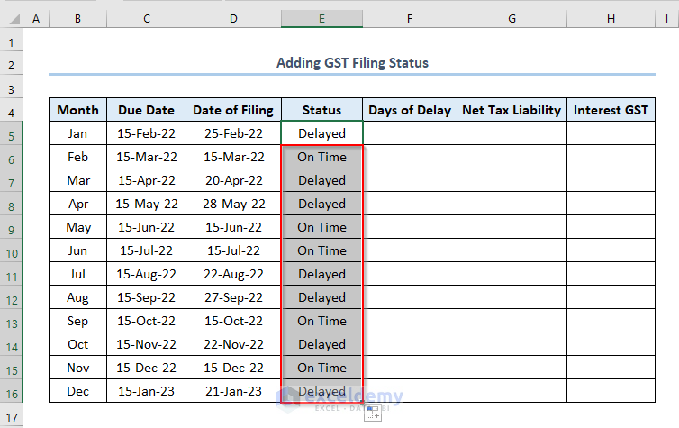
2. Adding GST Filing Status

In this step, we need to add GST Filing Status.

• Firstly, put the Date of Filing in D5:D16.

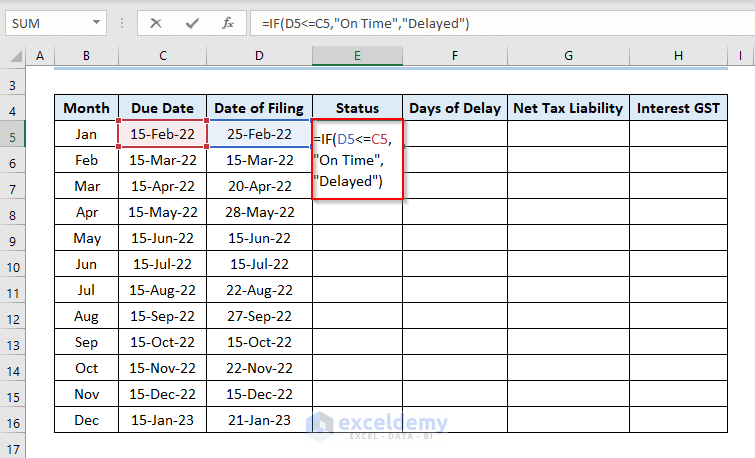
• Secondly, we need to calculate whether the Date of Filing has passed the due date or not. To do this, write the formula in the E5 cell like this.

Here, D5 and C5 refer to the first Date of Filing and the first Due Date respectively.

• Thirdly, press ENTER to get the output as Delayed.
• Fourthly, use the Fill Handle by dragging down the cursor while holding the right-bottom corner of the E5 cell like this.

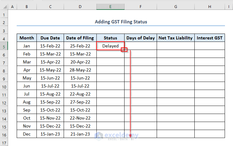
• Eventually, we’ll get the output like this.

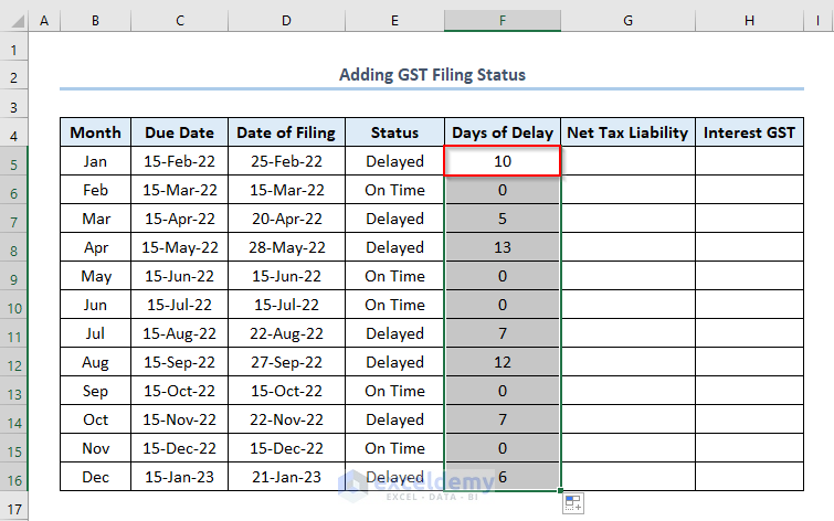
• Fifthly, we have to find the Days of Delay in Column F. So, write the formula in the F5 cell like this.

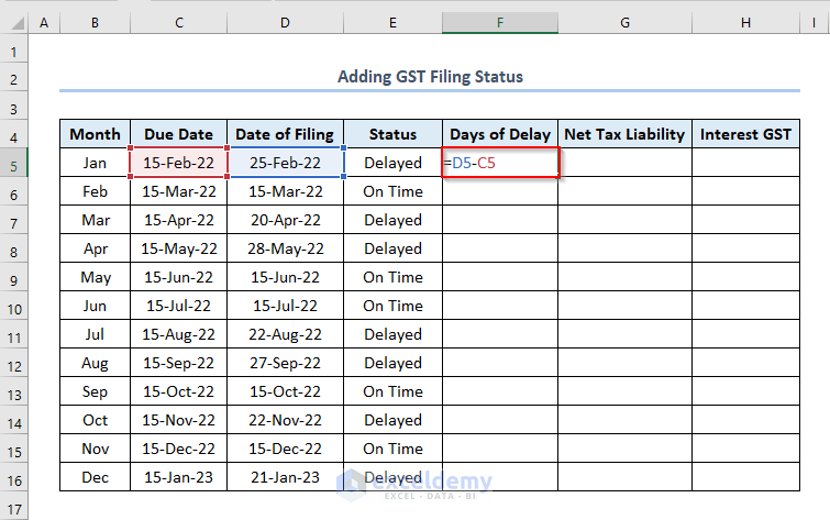
• Similarly, press ENTER and use the Fill Handle to get all the outputs like this.

Read More: Create Late Payment Interest Calculator in Excel and Download for Free

Similar Readings

• How to Use Cumulative Interest Formula in Excel (3 Easy Ways)
• Daily Loan Interest Calculator in Excel (Download for Free)
• How to Calculate Interest Between Two Dates Excel (2 Easy Ways)
• Car Loan Calculator in Excel Sheet – Download Free Template
• Bank Interest Calculator in Excel Sheet – Download Free Template

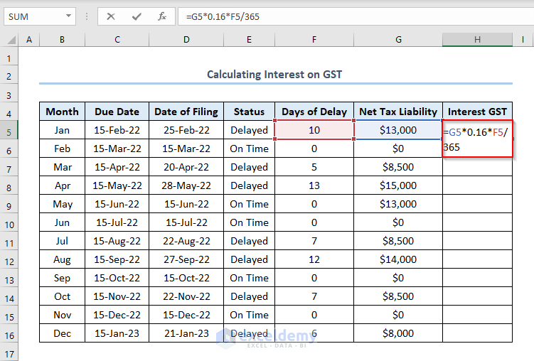
3. Calculating Interest on GST

To calculate interest on GST, we have to find out Net Tax Liability first. We need to assign Net Tax Liability for the concerned months. In our dataset, we have Net Tax Liability 8 times. For your case, find it from your notice and assign them as per the direction.

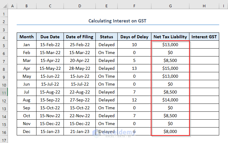
Interest will be counted for the months we haven’t paid the GST on time. We have considered the Interest Rate as 16%. You can proceed on your own.

• Secondly, in the H5 cell, write the formula to calculate Interest on GST.

Here, G5 and F5 refer to the first value of Net Tax Liability and Days of Delay.

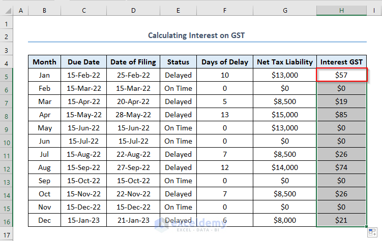
• Eventually, press ENTER and use the Fill Handle to get all the Interest GST as outputs.

Read More: Calculate Interest in Excel with Payments (3 Examples)

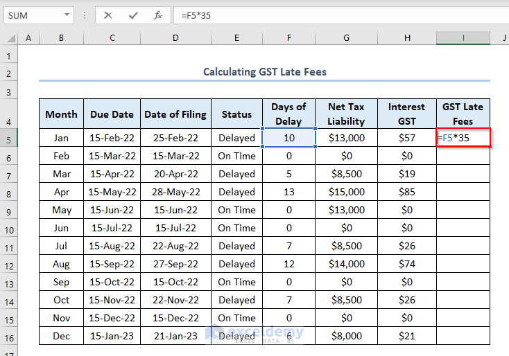
How to Calculate GST Late Fees and Total Payable Amount

We can also calculate GST Late Fees from the GST Interest Calculator. Now, calculate the GST Late Fees for the number of Delayed Days. We have considered Late Fees Per Day as 35.
So for getting the total late fees, multiply the number of Delayed Days by Late Fees Per Day.
In order to get the total late fees, write the following formula in the I5 cell like this.

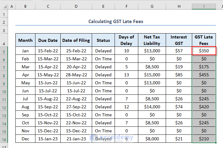
• Secondly, press ENTER and use the Fill Handle. So the outputs will be like this.

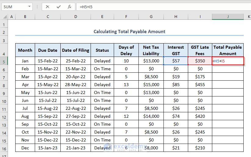
• Additionally, if we want to calculate the Total Payable Amount per month in the Column J, firstly write the formula in the J5 cell like this.

Here, H5 and I5 refer to the Interest GST and GST Late Fees in January respectively.

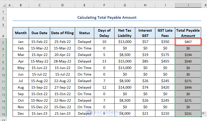
• Finally, press ENTER and use the Fill Handle.
• Consequently, we’ll get the Total Payable Amount for each month like this.

Read More: Perform Service Tax Late Payment Interest Calculation in Excel

Conclusion

That’s all about today’s session. And these are the ways to create a GST calculator in Excel. We strongly believe this article would be highly beneficial for you. Don’t forget to share your thoughts and queries in the comments section and explore our website Exceldemy, a one-stop Excel solution provider.

Related Articles

• How to Create Prejudgment Interest Calculator in Excel
• How to Make TDS Late Payment Interest Calculator in Excel
• Create Post-Judgment Interest Calculator in Excel (With 2 Cases)
• How to Calculate GPF Interest in Excel (with Easy Steps)
• How to Split Principal and Interest in EMI in Excel (with Easy Steps)
• Overdraft Interest Calculator in Excel (with Example)