Creating a Simple Interest Loan Calculator with a Payment Schedule in Excel – 5 Steps

Arithmetic Formula to Calculate the Simple Interest Loan

The Simple Interest Loan is the interest calculated by multiplying the initial borrowed amount -the Principal (p), the Rate of Interest (r), and Time (n). The arithmetic formula is:

I = p*n*r

I = Simple Interest (Total interest to be paid)
p= Principal Amount
n = Time elapsed
r = Rate of Interest

Consider a 5-year loan of $5000 with an annual interest of 15% . The calculation will be:

I = $5000 * 5 * 0.15 = $3750

The total amount of interest is $1500 in 5 years.

To calculate the Monthly Payable Interest, use the following formula.

Monthly Payable Interest = (p*r*)/12

In the previous example, the Monthly Payable Interest is:

= (p*r*)/12 = ($5000*0.15)/12 = $62.5

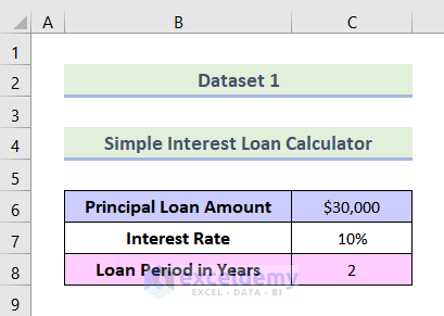
The dataset below showcases a bank loan of $30,000 taken at a 10% annual simple interest rate for 2 years.

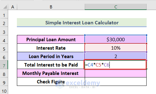
Step 1: Calculating the Total Interest to be Paid 

• Enter the following formula in C7.

C4 is the Principal Loan Amount, C5 refers to the Interest Rate, C6 represents the Loan Period in Years, and C7 is the Monthly Payable Interest.

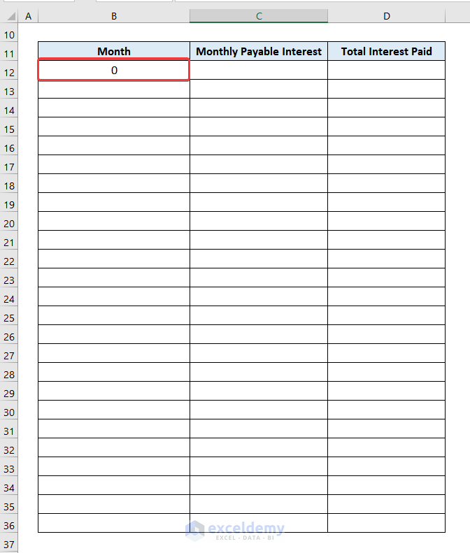
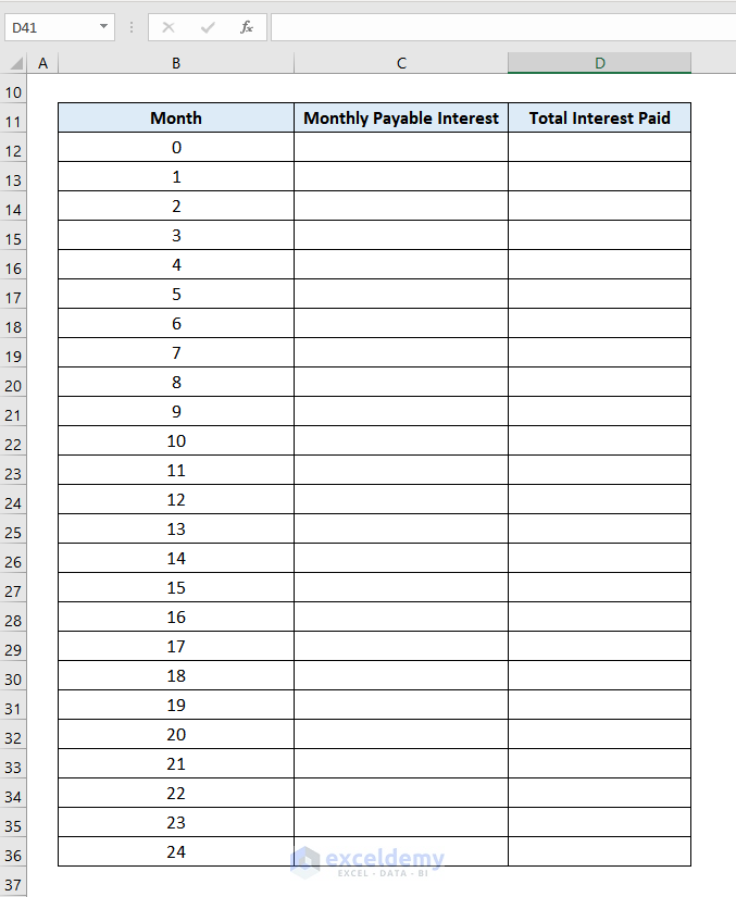
Step 2 – Determining the Number of Months to Repay the Loan

The month when the loan is taken is considered as Month 0.

• Enter 0 in B12.

• Enter the following formula in B13.

B12 refers to Month 0.

Formula Breakdown

• COUNT($B$12:B12) counts cells containing the value in B12 in column B.
• Checks the value is greater than the Loan Period*12 (Number of months) using the argument COUNT($B$12:B12)>$C$6*12 with a preceding IF function.
• If the above condition is true, the Loan Period has passed and a blank is returned. If the condition is false you are within the Loan Period and the cell value is increased by 1, using the following argument:

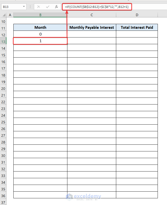
• Drag down the Fill Handle to see the result in the rest of the cells. The formula automatically stops at the end of the Loan Period.

Step 3 – Computing the Monthly Payable Interest

• Enter the formula in C8 to see the Monthly Payable Interest.

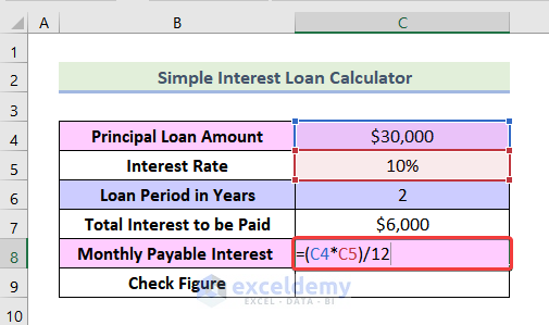
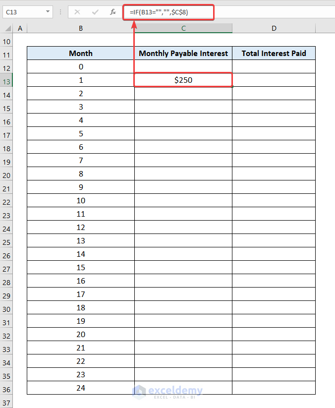
To add this value to the last month of the Loan Period:

• Use the following formula in C13.

C13 refers to the Monthly Payable Interest for the 1st month.

Formula Breakdown

• =IF(B13=””,””,$C$8) checks if the adjacent cell in column B is blank. If this condition is true, the Loan Period has passed and a blank is returned. If the condition is false, you are within the Loan Period and the Monthly Payable Interest ($C$8) is displayed.

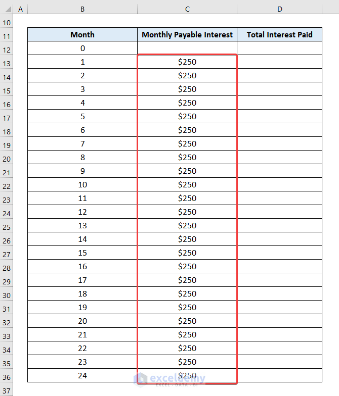
• Drag down the Fill Handle to see the result in the rest of the cells.

Step 4 – Calculating the Cumulative Total Interest Paid

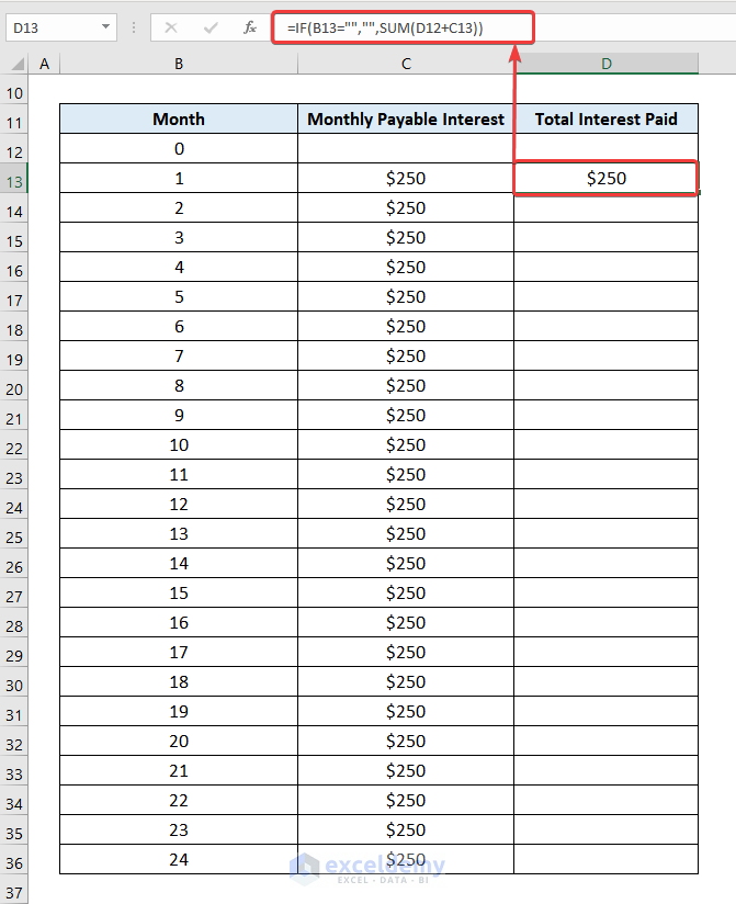
•  Use the following formula in C13.

D12 and D13 represent the Total Interest Paid in months 0 and 1.

• Drag down the Fill Handle to see the result in the rest of the cells.

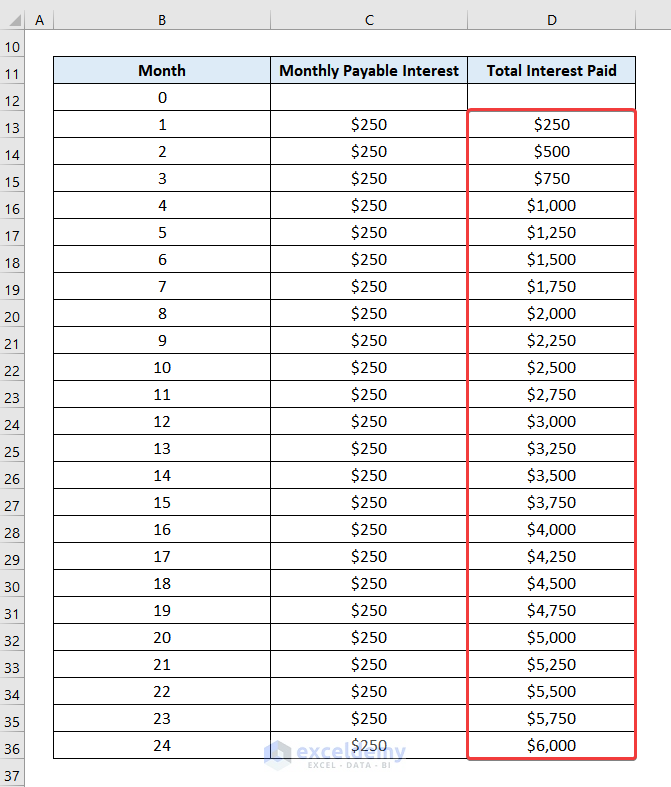
The simple interest loan calculator payment schedule is created.

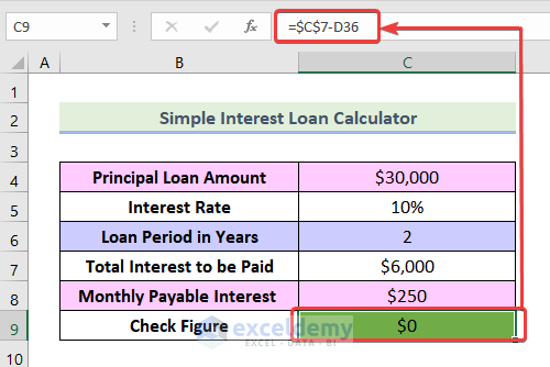
Step 5 – Checking the Figures in the Simple Interest Loan Calculator in Excel

Check whether the Total Interest Paid in the Payment Schedule matches the value in Step 1.

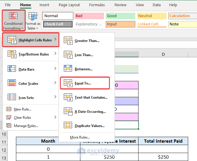
• Select C9 and click Conditional Formatting in the Home tab.
• Select Highlight Cell Rules.
• Choose Equal To.

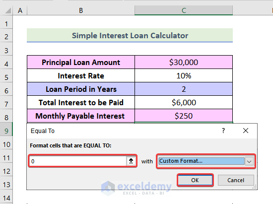
• In the Equal To dialog box, enter 0 as shown below.
• Select a formatting option.
• Click OK.

• In C9 use the following formula.

The cell is Green, which means the calculation in the Payment Schedule is correct.

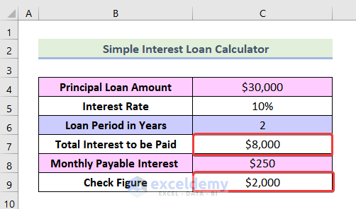
If the calculation was wrong (Total Interest to be Paid ≠ Total Paid Interest),  C9 wouldn’t be highlighted in green:

Below the Total Interest to be paid is $8000.  Total Interest to be Paid – Total Paid Interest = $2000. C9 is not highlighted in green, which indicates an error.

Things to Remember

• In Step 2, you need to use an Absolute Cell Reference in the starting point of the COUNT function ($B$12:B12) and in $C$6.
• In Step 3, you need to use an Absolute Cell Reference in $C$8.

Download Practice Workbook

Related Articles

• Car Loan Calculator in Excel Sheet
• Create Home Loan Calculator in Excel Sheet with Prepayment Option
• How to Create Loan Calculator with Extra Payments in Excel

<< Go Back to Finance Template | Excel Templates