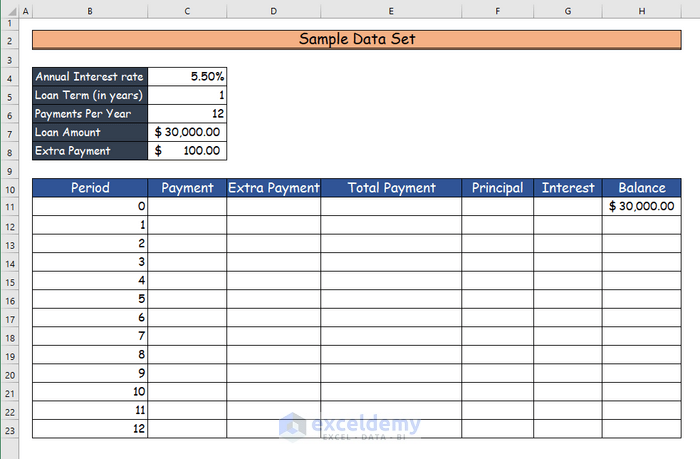
The sample dataset will be used to create an Excel loan calculator with extra payments.
Method 1- Applying the IFERROR Function to Create a Loan Calculator with Extra Payments in Excel
Steps:
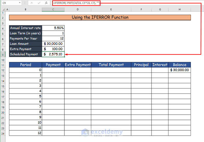
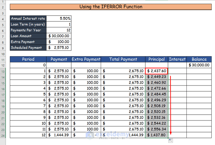
- Calculate the scheduled payment in C9.
- Use the following formula.
=IFERROR(-PMT(C4/C6, C5*C6, C7), "")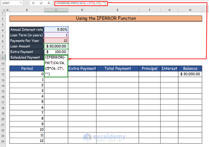
- Press Enter to see the scheduled payment in C9: $2,575.10.
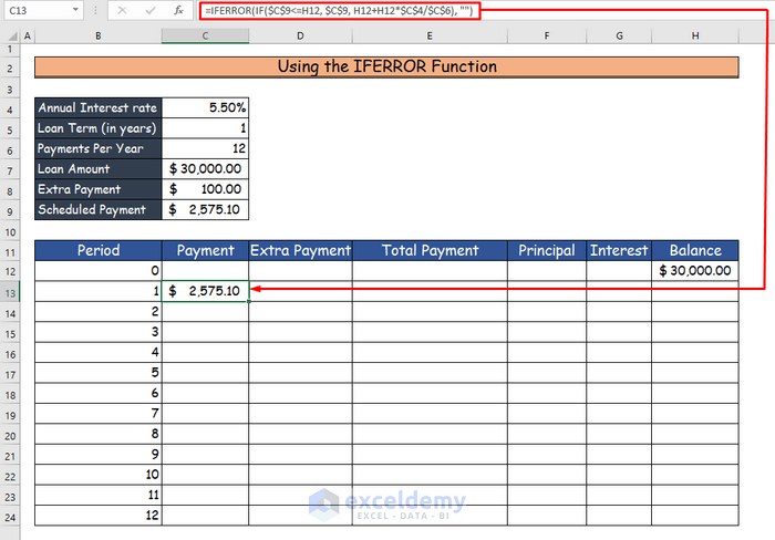
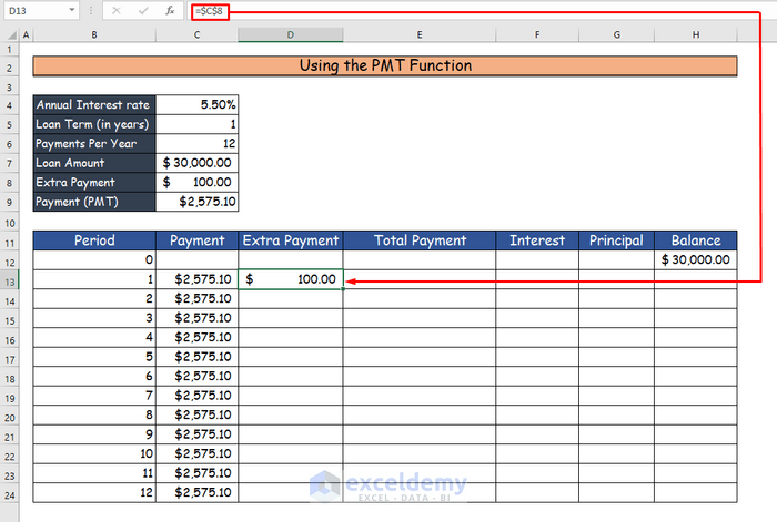
- Determine payment in C13.
=IFERROR(IF($C$9<=H12, $C$9, H12+H12*$C$4/$C$6), "")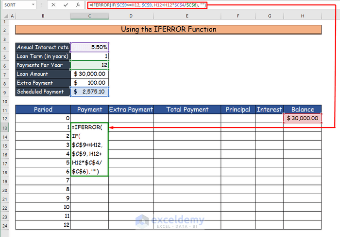
- Press Enter to see the payment for the first month in C13: $2575.10.
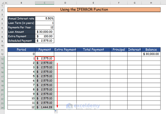
- AutoFill the formula in the rest of the cells in column C.
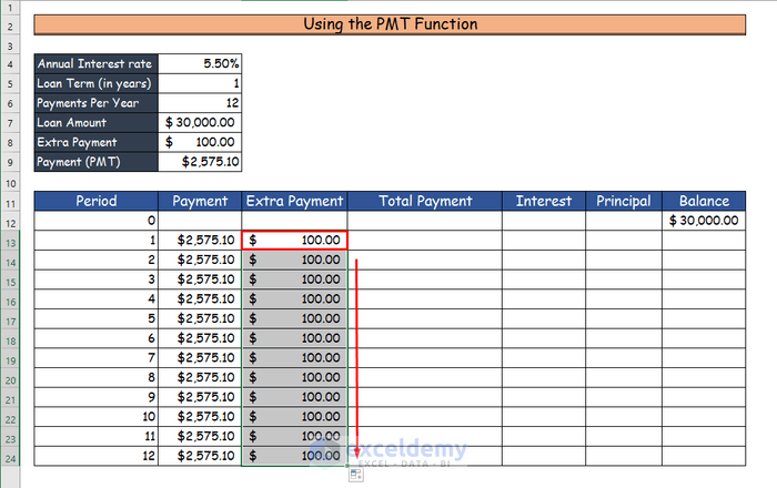
- Determine the extra payment in column D.
=IFERROR(IF($C$8<H12-F13,$C$8, H12-F13), "")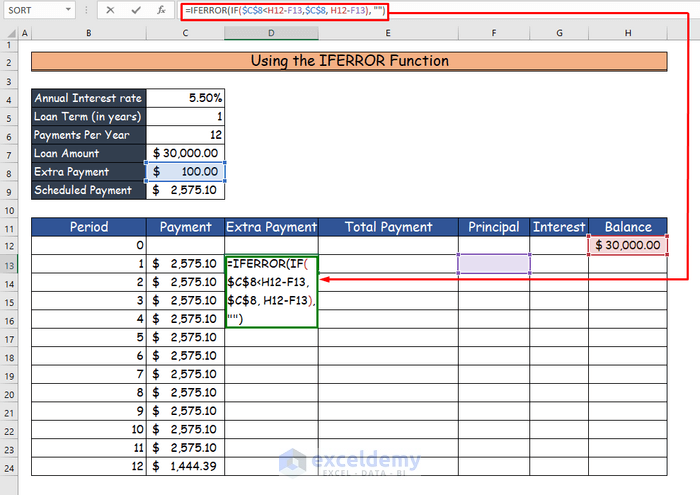
- Press Enter to see the extra payment for the first month in D13: $100.

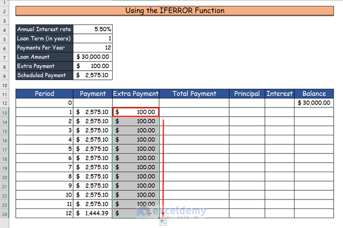
- Drag down the Fill Handle to see the result in the rest of the cells.
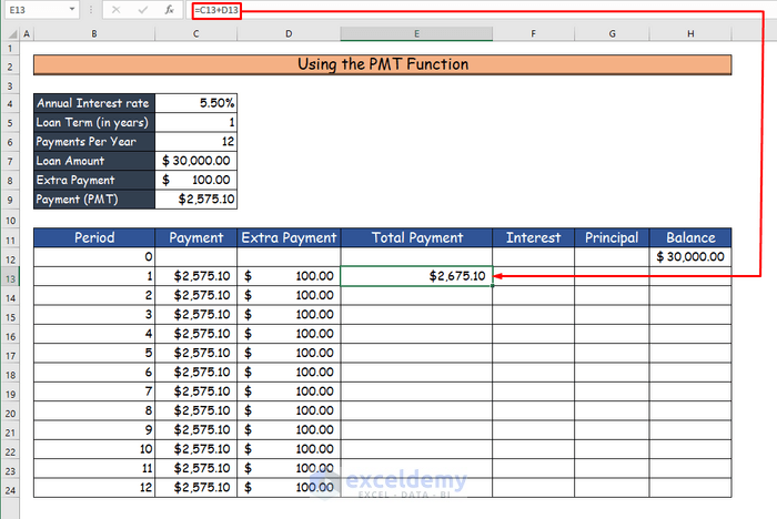
- Calculate the total payment in column E.
- Use the formula below.
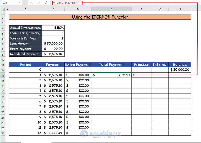
=IFERROR(C13+D13, "")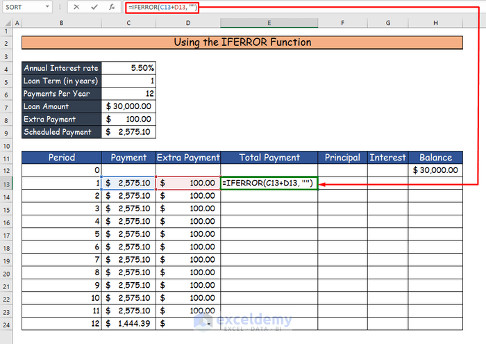
- Press Enter to see the total payment for the first month in E13: $2,675.10.
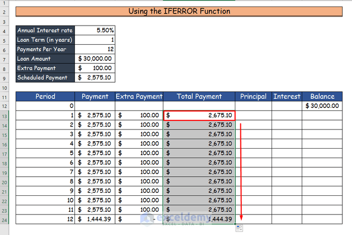
- Drag down the Fill Handle to see the result in the rest of the cells.
- Determine the principal in column F.
=IFERROR(IF(C13>0, MIN(C13-G13, H12), 0), "")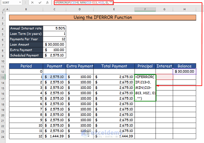
- Press Enter to see the principal for the first month in F13: $2,437.60.

- Drag down the Fill Handle to see the result in the rest of the cells.
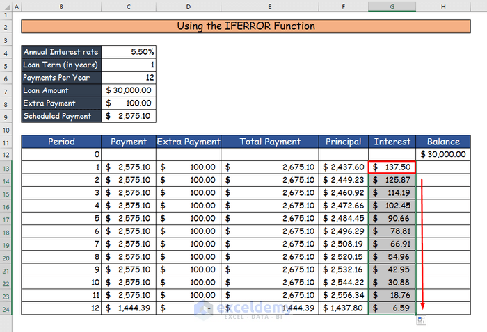
- Calculate the interest.
- Use the following formula.
=IFERROR(IF(C13>0, $C$4/$C$6*H12, 0), "")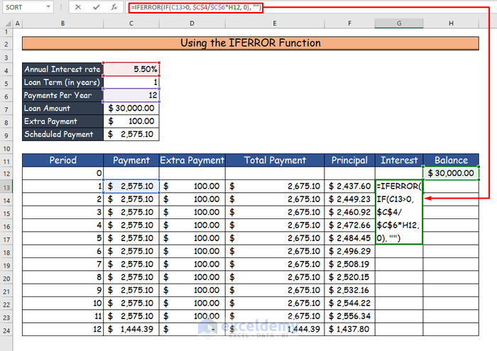
- Press Enter to see the value of the interest in G13: $137.50.

- Drag down the Fill Handle to see the result in the rest of the cells.
- Calculate the balance in column H.
=IFERROR(IF(H12 >0, H12-F13-D13, 0), "")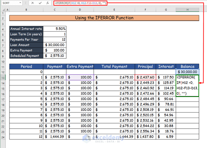
- Press Enter to see the value of the balance in H13: $ 27,462.40.
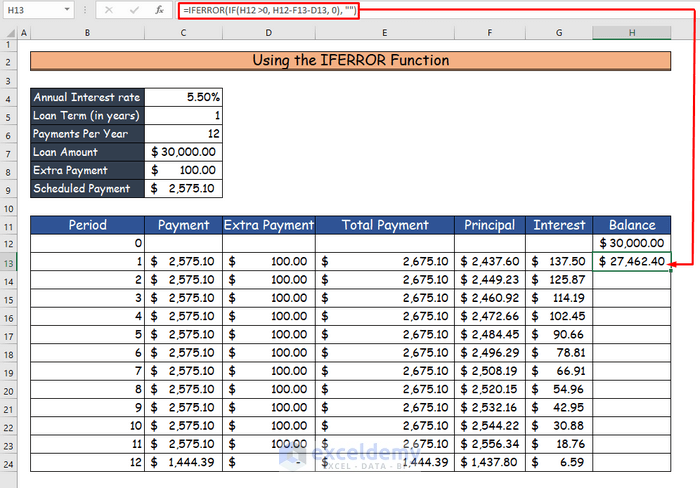
- Drag down the Fill Handle to see the result in the rest of the cells.
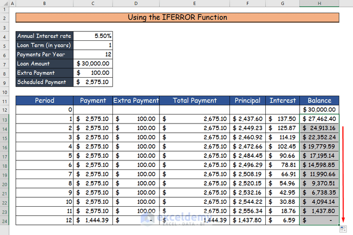
This is the output.
Method 2 – Combining the PMT, IPMT, and PPMT Functions to Create an Excel Loan Calculator with Extra Payments
Steps:
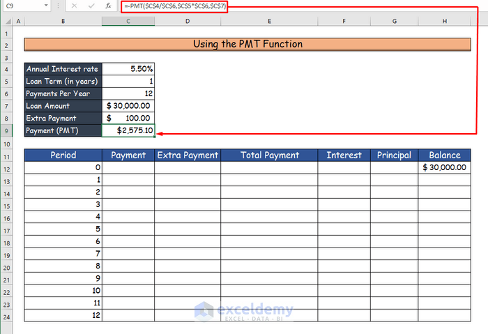
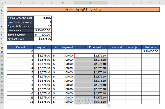
- Calculate the payment (PMT) in C9.
- Use the following formula.
=-PMT($C$4/$C$6,$C$5*$C$6,$C$7)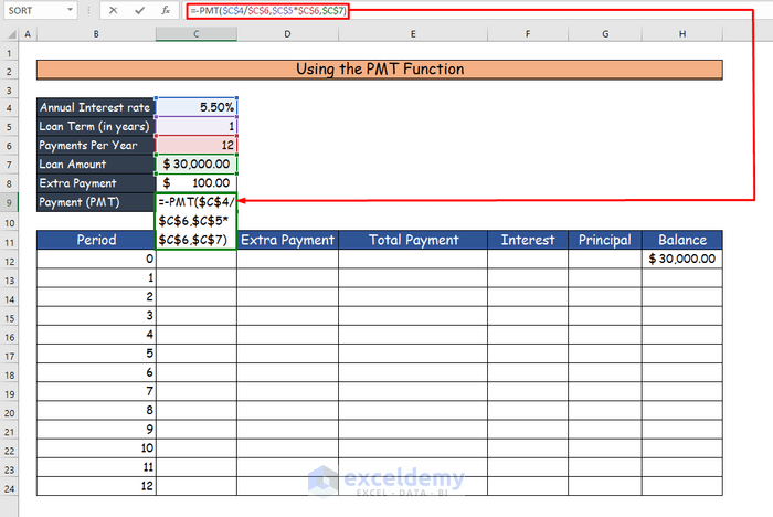
- Press Enter to see the scheduled payment in C9: $2,575.10.
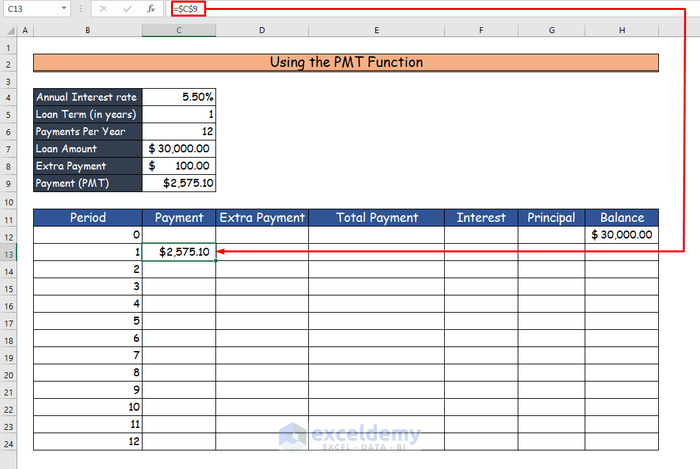
- Add the value of payment to C13, which is equal to C9.
=$C$9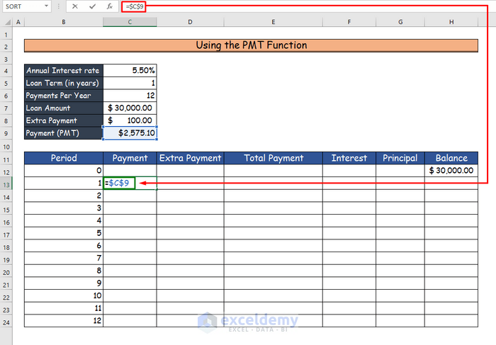
- Press Enter to see the payment for the first month in C13: $2575.10.
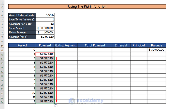
- Drag down the Fill Handle to see the result in the rest of the cells.
- Enter the value of the extra payment in column D, which is equal to C8.
=$C$8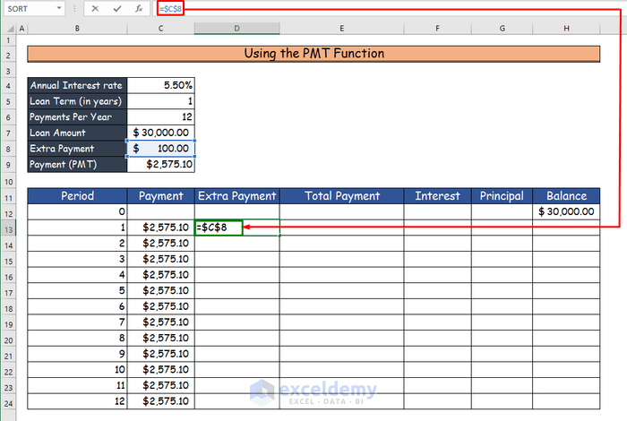
- Press Enter to see the extra payment for the first month in D13: $100.
- Drag down the Fill Handle to see the result in the rest of the cells.
- Calculate the total payment in column E by entering the following formula.
=C13+D13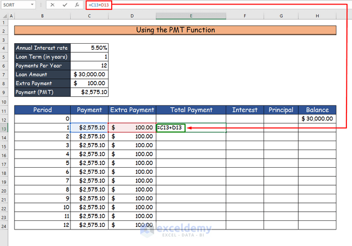
- Press Enter to see the total payment for the first month in E13: $2,675.10.
- Drag down the Fill Handle to see the result in the rest of the cells.
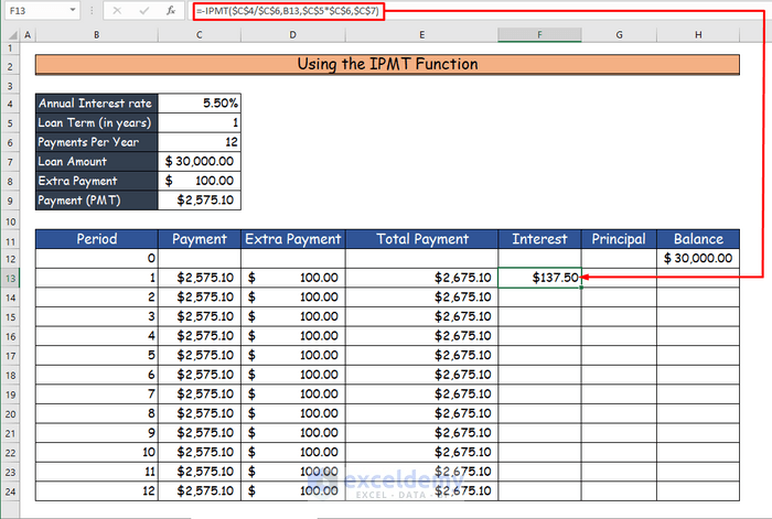
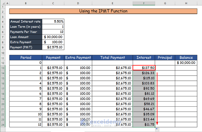
- Determine the interest in column F using the formula below.
=-IPMT($C$4/$C$6,B13,$C$5*$C$6,$C$7)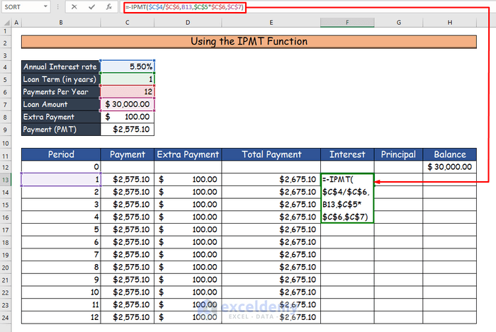
- Press Enter to see the interest for the first month in F13: $137.50.
- Drag down the Fill Handle to see the result in the rest of the cells.
- Calculate the principal in column G. Enter the formula.
=-PPMT($C$4/$C$6,B13,$C$5*$C$6,$C$7)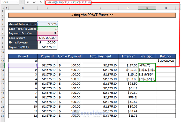
- Press Enter to see the value of the principal in G13: $2437.60.

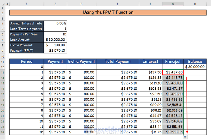
- Drag down the Fill Handle to see the result in the rest of the cells.
- Calculate the balance in column H by using the following formula.
=H12-G13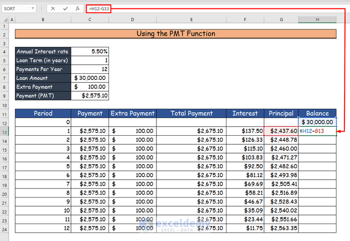
- Press Enter to see the value of the balance in H13: $ 27,562.40.

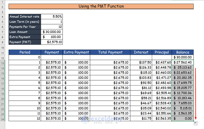
- Drag down the Fill Handle to see the result in the rest of the cells.
This is the output.
Notes:
- Use a minus (-) sign before the PPT, IPMT, and PPMT functions. The value from the formula will be positive and easier to calculate.
- Use an absolute cell reference.
Download Practice Workbook
Download the free Excel workbook here.
Related Articles
- Create Home Loan Calculator in Excel Sheet with Prepayment Option
- Excel Simple Interest Loan Calculator with Payment Schedule
- Car Loan Calculator in Excel Sheet
<< Go Back to Loan Calculator | Finance Template | Excel Templates
Get FREE Advanced Excel Exercises with Solutions!
