Method 1 – Using the AVERAGEIF Function in Excel
STEPS:
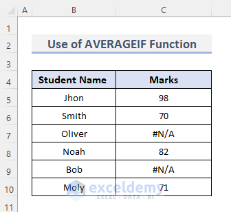
- We need to create a dataset. We have some students’ names and their marks for a subject. We want to compute the average of those students’ marks. Some of the students were absent during the exam period that’s why they have the #N/A value in their mark column.
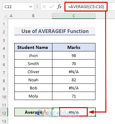
- Select cell C12 and enter the formula :
=AVERAGE(C5:C10)- Press Enter.
- Unfortunately, we will get a #N/A error.
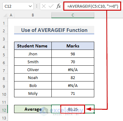
- To avoid this, we are using the AVERAGEIF function.
- Choose cell C12 and insert the formula:
=AVERAGEIF(C5:C10, ">=0")- Press Enter.
You will get the accurate average value without any errors.
Read More: [Fixed!] AVERAGE Formula Not Working in Excel
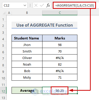
Method 2 – Using the Excel AGGREGATE Function for Ignoring #N/A Error Values
STEPS:
- Use the same dataset as the previous method.
- Select cell C12 and enter the following formula:
=AVERAGE(C5:C10)- Press Enter.
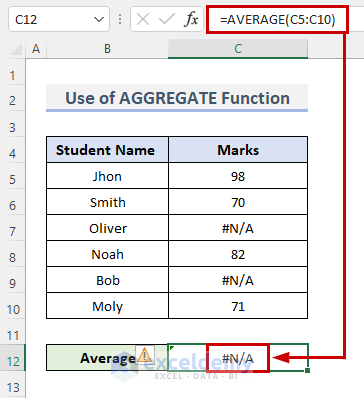
We get an error #N/A.
- Use the AGGREGATE function to prevent this.
- Choose cell C12 and enter the formula below:
=AGGREGATE(1,6,C5:C10)- Press Enter.
- You will obtain the average number accurately and without error.
Read More: How to Fix Divide by Zero Error for Average Calculation in Excel
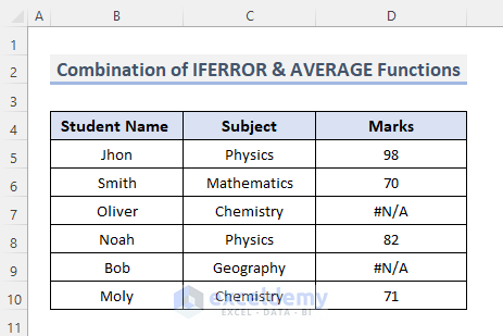
Method 3 – Combining IFERROR and AVERAGEIF Functions to Avoid Error When Getting Average
STEPS:
- We want to determine those students’ average grades. Some students missed the exam session, so their mark column has a #N/A value.
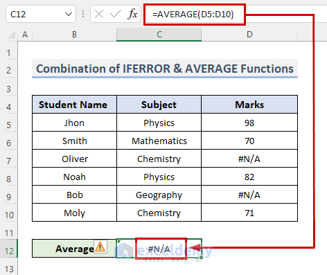
- Use the AVERAGE function to determine the average.
- Choose cell C12 and enter the following formula:
=AVERAGE(D5:D10)- Press Enter.
- Unfortunately, we will encounter an error of #N/A.
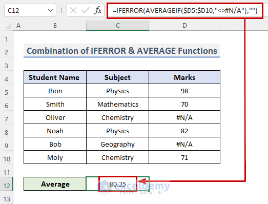
- We can prevent this by combining the IFERROR and AVERAGE functions.
- Choose cell C12 and enter the following formula:
=IFERROR(AVERAGEIF($D5:$D10,"<>#N/A"),"")- Press Enter.
- You will have an accurate average number.
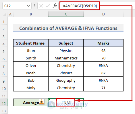
Method 4 – Merging the AVERAGE and IFNA Functions to Ignore #N/A Error in Excel
STEPS:
- Use the same dataset.
- Select the cell C12 and enter the following formula:
=AVERAGE(C5:C10)- Press Enter.
- But we get an error.
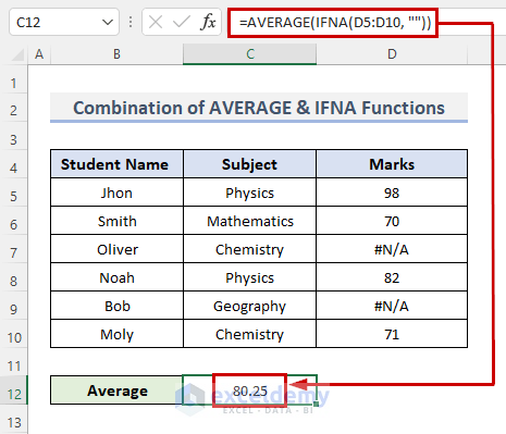
- We are applying the AVERAGE & IFNA functions to prevent this.
- Choose cell C12 and enter the following formula:
=AVERAGE(IFNA(D5:D10, ""))- Press Enter.
- You will get the precise average.
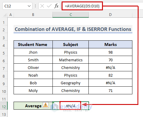
Method 5 – Using a Combination of AVERAGE, IF & ISERROR Functions
STEPS:
- Use the same dataset.
- Select the cell C12 and enter the following formula:
=AVERAGE(C5:C10)- Press Enter.
- But an error occurs.
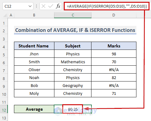
- To avoid this, we are using the combination of AVERAGE, IF & ISERROR functions.
- Choose cell C12 and enter the following formula:
=AVERAGE(IF(ISERROR(D5:D10),"",D5:D10))- Press Enter.
- You will arrive at an accurate average.
Things to Keep in Mind
- While inputting any function, the function name must be enclosed in empty brackets. If not, Excel will fail to identify it as a function.
- Alternatively, we can enter the value #N/A into a cell. For compatibility with other spreadsheet programs.
Download the Practice Workbook
You can download the workbook to practice.
Related Articles
- How to Average a Column in Excel
- How to Calculate Average of Multiple Columns in Excel
- How to Calculate Average of Multiple Ranges in Excel
- How to Find Average of Specific Cells in Excel
- How to Find Average with Blank Cells in Excel
- How to Average Only Visible Cells in Excel
- How to Exclude a Cell in Excel AVERAGE Formula
- How to Average Every Nth Row in Excel


Hi there, why would the =IFERROR(AVERAGEIF($D5:$D10,”#N/A”),””) need a dollar sign before the column?
Hello Liz,
You can avoid the absolute reference ($ sign). Here absolute reference is used so that it can avoid error if anyone copy the formula in another cell.
Regards
ExcelDemy