Method 1 – Using the AVERAGEIF Function to Find the Average of Specific Cells in Excel
1.1 Using AVERAGEIF and Comparison Operator
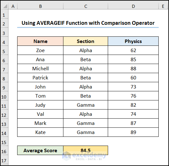
Find the average of the Physics scores that are greater than or equal to 75 using the comparison operator.
Steps:
- Go to the C16 cell and enter the following formula.
=AVERAGEIF(D5:D14,">="&75)Cells D5:D14 represent the marks in Physics while the “>=”&75 specify the criterion which is greater than or equal to 75.
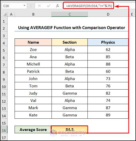
The results should look like the image given below.
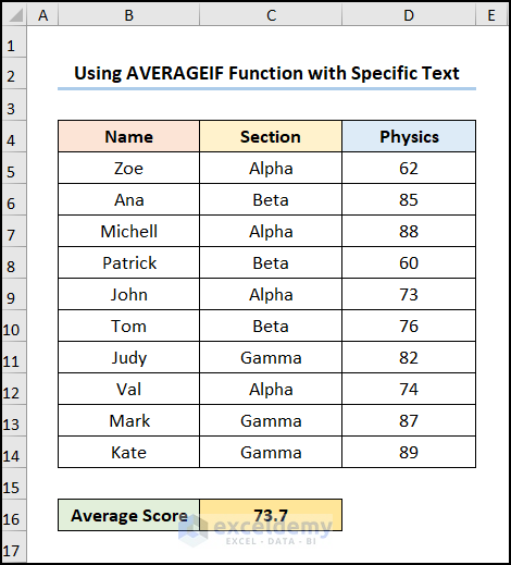
1.2 Applying AVERAGEIF to Match Specific Text
Steps:
- Select cell C16 and enter the following formula.
=AVERAGEIF(C5:C14,"*Beta*",D5:D14)Ranges C5:C14 and D5:D14 refer to the Section and Physics columns respectively. Meanwhile, the “*Beta*” represents the criteria to match. As a note, the asterisk (*) character before and after Beta indicates an exact match.
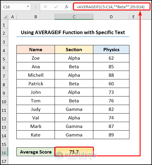
The results should look like the picture given below.
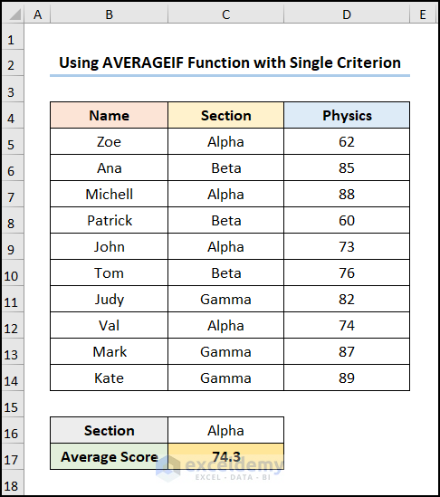
1.3 Using AVERAGEIF with Single Criteria
Steps:
- Select cell C17 and enter the following formula.
=AVERAGEIF(C5:C14,C16,D5:D14)Ranges C5:C14 and D5:D14 represent the Section and Physics columns respectively. Cell C16 points to Section Alpha which is given criterion.
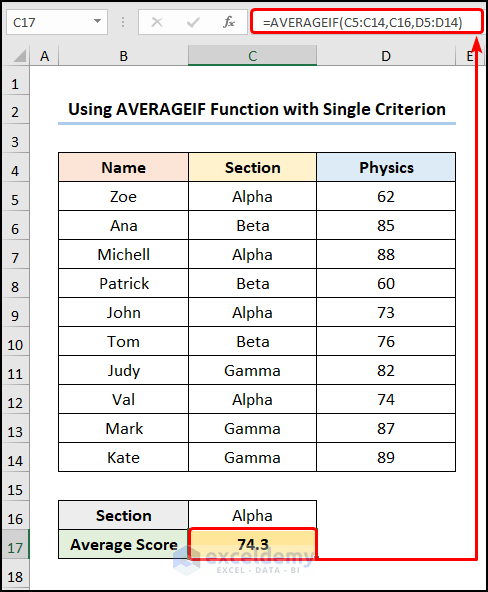
The output should look like shown in the image below.
Read More: How to Calculate Average of Multiple Ranges in Excel
Method 2 – Using AVERAGEIFS Function
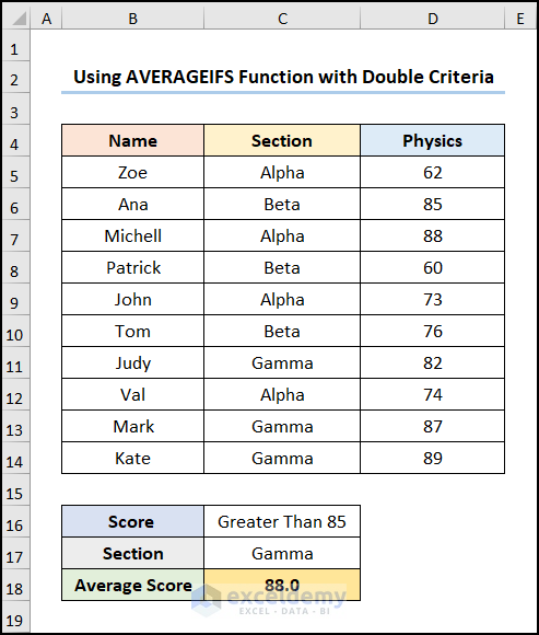
2.1 Employing AVERAGEIFS with Double Criteria
Steps:
- Select cell C18 and enter the following formula.
=AVERAGEIFS(D5:D14,C5:C14,C17,D5:D14,">="&85)- AVERAGEIFS(D5:D14,C5:C14,C17,D5:D14,”>=”&85) → finds average for the cells specified by a given set of conditions or criteria. D5:D14 is the average_range argument which is the Physics column. C5:C14 is the criteri_range1 argument which refers to the Section column and the C17 is the criteria1 argument which is Section Gamma. Following this, D5:D14 is the criteri_range2 argument which refers to the Physics column, and the “>=”&85 is the criteria2 argument which represents the values greater than and equal to 85.
- Output → 88.0
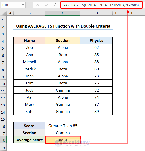
The results should look like the image below.
Read More: How to Calculate Average of Multiple Columns in Excel
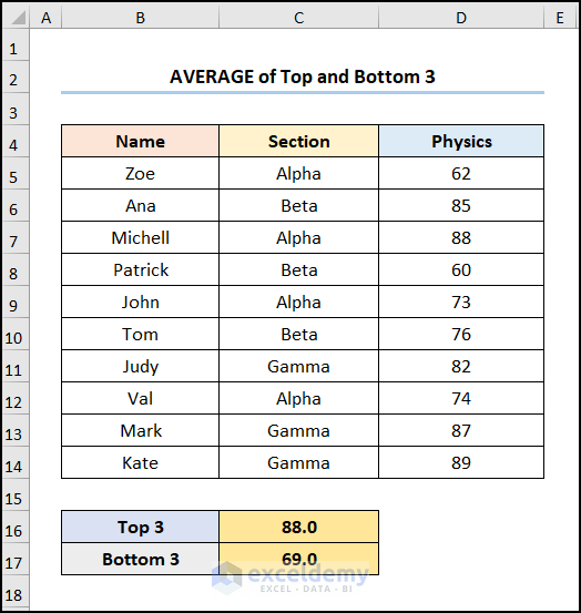
2.2 Combining AVERAGE, LARGE, and SMALL Functions to Calculate Top and Bottom 3 Averages
Steps:
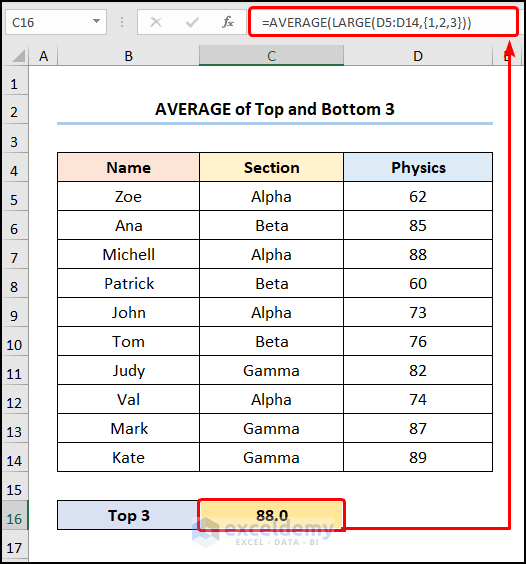
- Select cell C16 and enter the following
=AVERAGE(LARGE(D5:D14,{1,2,3}))- LARGE(D5:D14,{1,2,3}) → returns the nth largest value in a dataset. Here, range D5:D14 represents the Physics column. {1,2,3} refers to the 3 of the largest values in the Physics column.
- Output → 89, 88, 87
- AVERAGE(LARGE(D5:D14,{1,2,3})) → becomes
- AVERAGE(89, 88, 87) → returns the average of the arguments. Here, the values of 89, 88, and 87 are summed and divided by 3 to return their respective average.
- Output → 88.0
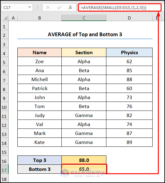
- Select cell C17 and enter in the following formula.
=AVERAGE(SMALL(D5:D15,{1,2,3}))- SMALL(D5:D14,{1,2,3}) → returns the nth smallest value in a dataset. Here, range D5:D14 represents the Physics column. {1,2,3} refers to the 3 of the smallest values in the Physics column.
- Output → 60, 62, 73
- AVERAGE(SMALL(D5:D14,{1,2,3})) → becomes
- AVERAGE(60, 62, 73) → returns the average of the arguments. Here, the values of 60, 62, and 73 are summed and divided by 3 to return their respective average.
- Output → 65.0
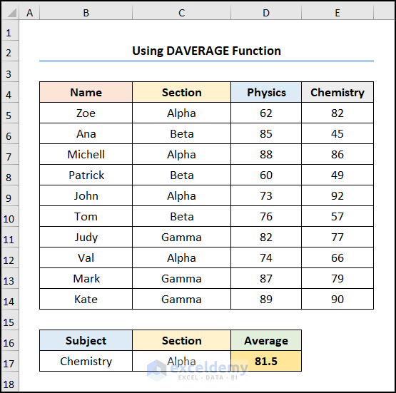
Method 3 – Using DAVERAGE Function to Find Average of Specific Cells in Excel
Steps:
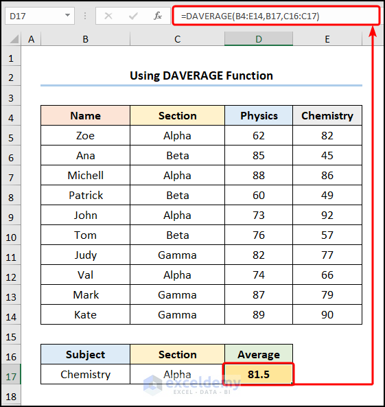
- Select cell D17 and enter the following formula.
=DAVERAGE(B4:E14,B17,C16:C17)- DAVERAGE(B4:E14, B17, C16:C17) → averages the values in a database that match the specified conditions. B4:E14 is the database argument that represents all the cells in the dataset. B17 is the field argument, which refers to the Chemistry subject. Lastly, the C16:C17 is the criteria argument, which is Section Alpha.
- Output → 81.5
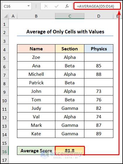
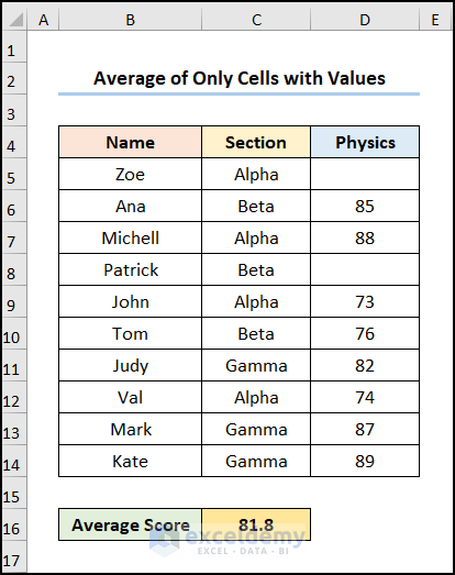
Calculate the Average of Only Cells with Values in Excel
Steps:
- Select cell C16 and enter the following formula.
=AVERAGEA(D5:D14)Range D5:D14 represents the scores in Physics.
Read More: How to Average Only Visible Cells in Excel
Download Practice Workbook
You can download the practice workbook from the link below.
Related Articles
- How to Average a Column in Excel
- How to Find Average with Blank Cells in Excel
- How to Exclude a Cell in Excel AVERAGE Formula
- How to Average Every Nth Row in Excel
- How to Fix Divide by Zero Error for Average Calculation in Excel
- How to Ignore #N/A Error When Getting Average in Excel
- [Fixed!] AVERAGE Formula Not Working in Excel
<< Go Back to Conditional Average | Calculate Average | How to Calculate in Excel | Learn Excel
Get FREE Advanced Excel Exercises with Solutions!
