How to Average Filtered Data in Excel (2 Easy Methods)

Filtering data is one of the most useful tools of Microsoft Excel. But when it comes to averaging those filtered data, some people may find it problematic as the AVERAGE function consider not only the filtered data but also the hidden data in the specified range. In this article, we will learn how to average filtered data in Excel. So let’s begin!

Download Practice Workbook

Download this practice workbook to exercise while you are reading this article.

2 Useful Methods to Average Filtered Data in Excel

We will demonstrate two effective methods to average filtered data in excel with appropriate illustrations. To demonstrate, we will consider an example where we have a list of expenditures within different categories shown in the picture below.

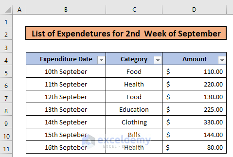
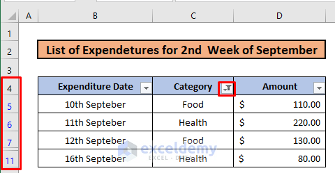
Suppose we filter the list based on the category Food and Health. So our filtered list would look like the figure below.

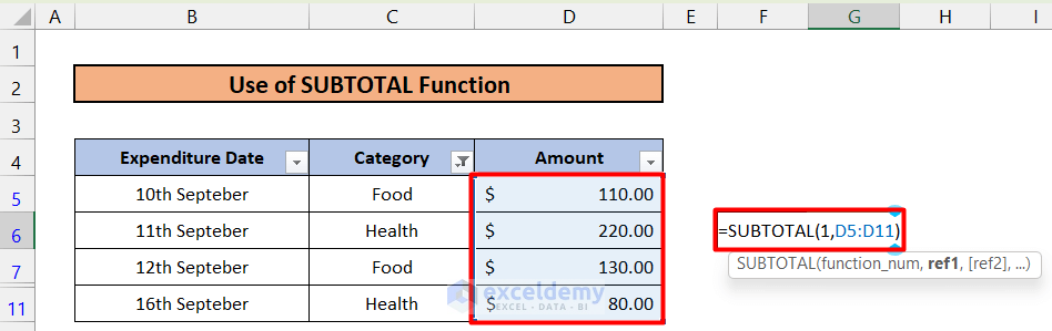
Now, we want to determine the average of the filtered data. To do that, let’s look at our first method.

1. Use of SUBTOTAL Function to Average Filtered Data in Excel

In this method, we will use the SUBTOTAL function. This function allows us to calculate sum, average, maximum, minimum, and many other parameters in a filtered range. It only counts the visible data and ignores the hidden data. The steps for applying this function are given below.

Steps:

• Select any cell and input the following formula

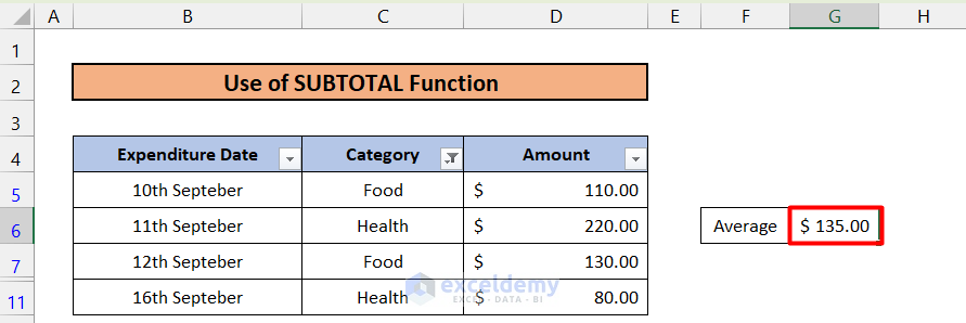
Here,

• 1 is for calculating Average.
• D5:D11 is the filtered range from where the average will be calculated.

• Now press Enter, and you will get the average value of the filtered cells,  which is135.

Read More: How to Average a Column in Excel (7 Easy Methods)

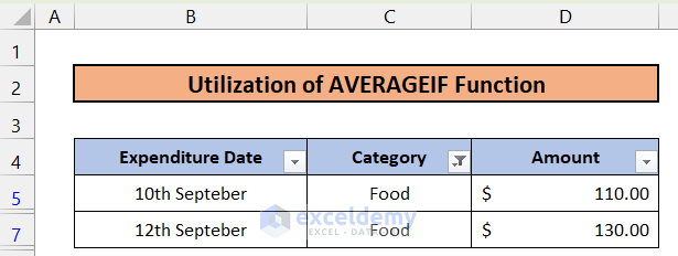
2. Utilize AVERAGEIF Function to Average Filtered Data in Excel

The problem with the SUBTOTAL function is that when you undo filtering of the range, the average will get changed. To fix the issue, we can use the AVERAGEIF Function so that our calculated average remains unchanged. But this time, we can only filter one category. So either Food or Health should be filtered, not both. Here, we will filter only the Food category.

Now to calculate the average of these filtered cells, follow the steps below:

Steps:

• Select any cell and input the following formula

Here,

• C5:C7 is the criteria range.
• “Food” is the Criteria.
• D5:D7 is the range of cells to be averaged.

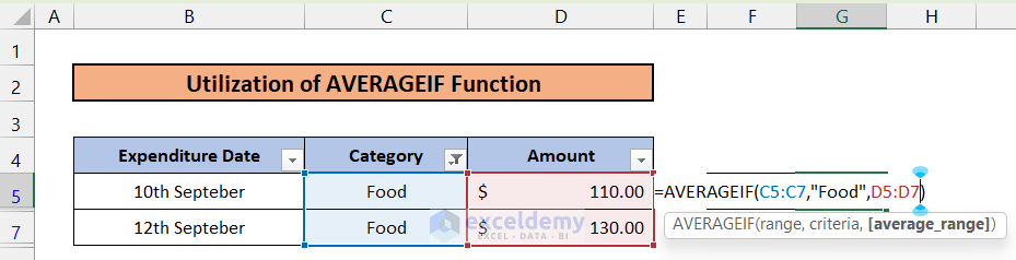
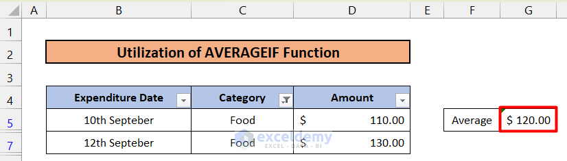
• Now press Enter, and you will have the average of the filtered cells.

• This time even if you undo the filtering of the range, the average will be unchanged.

Read More: How to Calculate Average of Multiple Columns in Excel (6 Methods)

Things to Remember

• The result from the SUBTOTAL function is subject to change as the filtered range changes.
• The AVERAGEIF function takes only one criterion to calculate the average of filtered cells.

Conclusion

That is the end of this article. If you find this article helpful, please share this with your friends. Moreover, do let us know if you have any further queries. Finally, please visit Exeldemy for more exciting articles on Excel.

Related Articles

• How to Calculate Average of Multiple Ranges in Excel (3 Methods)
• Fix Divide by Zero Error for Average Calculation in Excel
• How to Calculate Average of Text in Excel (2 Ways)
• Calculate Moving Average for Dynamic Range in Excel (3 Examples)
• How to Calculate Average Percentage Increase in Excel
• Calculate Average Numbers in Excel (9 Handy Methods)
• How to Do Subtotal Average in Excel (5 Suitable Ways)