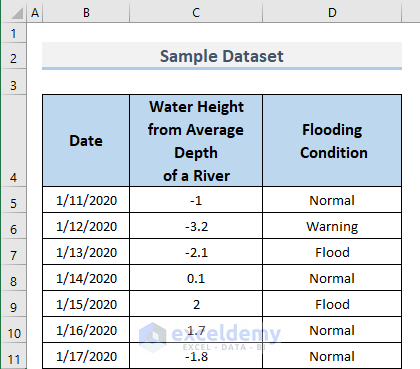
We have created a column in Excel with positive and negative numbers like Water Height from the Average Depth of a River in the range C4:C11. We have a Date column in range B4:B11 and a Flooding Condition column in range D4:D11 related to the water height of that particular river.
Method 1 – Use the AVERAGE Function to Average Negative and Positive Numbers
Steps:
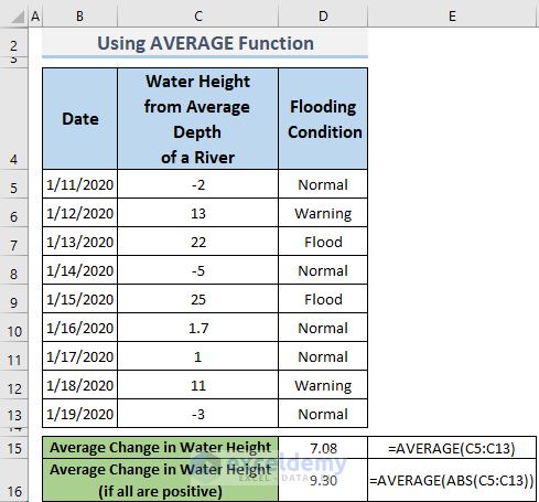
- The Average Change in Water Height is found by using the following formula.
=AVERAGE(C5:C13)- Range C5:C13 has positive and negative numbers.
- The AVERAGE function will add the positive and negative numbers and divide them by the available numbers of water height data in this case the number is 9.
- We used the following formula to find the average using the ABS function:
=AVERAGE(ABS(C5:C13))- Range C5:C13 has positive and negative numbers.
- ABS (C5:C13) returns {2;13;22;5;25;1.7;1;11;3} which means ABS turns all negative values into positive values.
- These positive values {2;13;22;5;25;1.7;1;11;3} are the input of the AVERAGE function that will add the numbers and divide them by the number of water height data points.
Read More: How to Average Filtered Data in Excel
Method 2 – Using the AVERAGE and IF Functions
Steps:
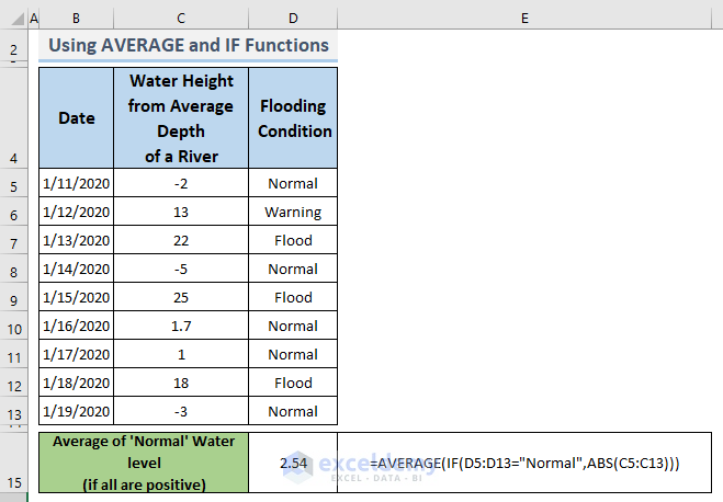
- We need the water height data when the Flooding Condition is Normal. We will use the following formula in Excel:
=AVERAGE(IF(D5:D13="Normal",ABS(C5:C13)))- Range C5:C13 has positive and negative numbers.
- IF (D5:D13=”Normal”, then return ABS (C5:C13)) which will be {2; FALSE; FALSE;5; FALSE;1.7;1; FALSE;3}.
- The AVERAGE function will add the numbers and divide them by the available numbers of water height data points.
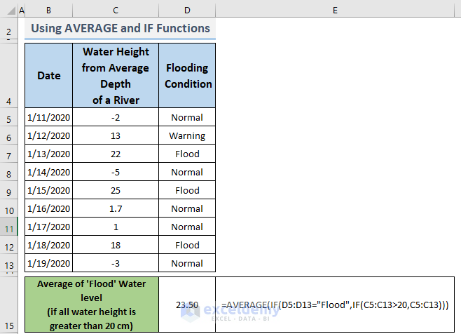
- We need the water height data when the Flooding Condition is flooded and the corresponding water height is also greater than 20. We will use the following formula in Excel.
=AVERAGE(IF(D5:D13="Flood",IF(C5:C13>20,C5:C13)))- Range C5:C13 has positive and negative numbers.
- IF (C5:C13>20, C5:C13) which will be {FALSE; FALSE;22; FALSE;25; FALSE; FALSE; FALSE; FALSE}.
- IF (D5:D13=”Flood”, IF (C5:C13>20, C5:C13)) will be the input of the AVERAGE function which will look like the following formula: =AVERAGE ({FALSE; FALSE;22; FALSE;25; FALSE; FALSE; FALSE; FALSE}).
- The AVERAGE function will add the numbers and divide them the applicable number of data points.
We used the statistical function called AVERAGE function in Excel which returns the average value of data with the combination of the IF function. Excel has a built-in function that can do the same job more easily and spontaneously.
Alternative Steps:
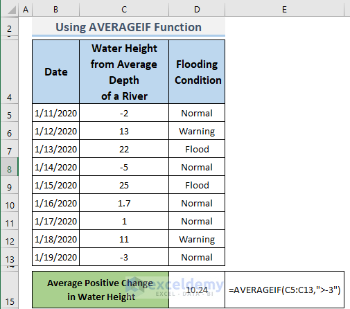
- We need the water height data when the Flooding Condition is flooded and the corresponding water height is also greater than 20. Apply the following formula.
=AVERAGEIF(C5:C13,">-3")range = C5:C13
criteria = “>-3”
- The AVERAGEIF function will add the numbers and divide them by the available numbers of water height data.
Read More: How to Calculate Average of Text in Excel
Download the Practice Workbook
Related Articles
- How to Do Subtotal Average in Excel
- How to Calculate Sum & Average with Excel Formula
- How to Calculate Average and Standard Deviation in Excel
- How to Calculate Average Deviation in Excel Formula
- How to Calculate Average Excluding Outliers in Excel
<< Go Back to Calculate Average in Excel | How to Calculate in Excel | Learn Excel
Get FREE Advanced Excel Exercises with Solutions!
