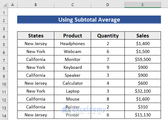
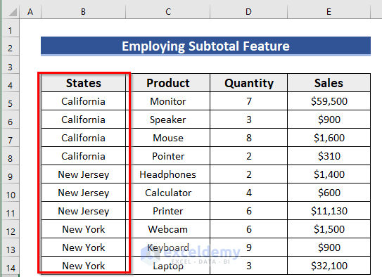
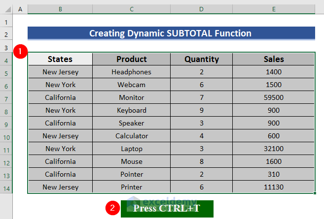
This is the sample dataset, showcasing States, Product, Quantity, and Sales.
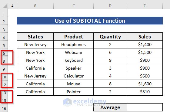
Method 1 – Using the SUBTOTAL Function Including Hidden Values
Rows 7,11, and 14 are hidden.
Steps:
- Select a blank cell: E16 to keep the result.
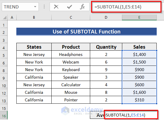
- Use the formula in E16.
=SUBTOTAL(1,E5:E14)1 is the AVERAGE function and E5:E14 is the data range. This function will consider all the cells even the hidden ones.
- Press ENTER to see the result.
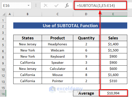
This is the output.
Read More: How to Calculate Sum & Average with Excel Formula
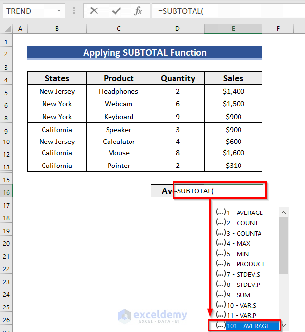
Method 2 – Applying the SUBTOTAL Function Excluding Hidden Values
101 is the 1st argument of the SUBTOTAL function to perform an operation excluding hidden values.
Steps:
- Select a blank cell: E16 and enter the following formula.
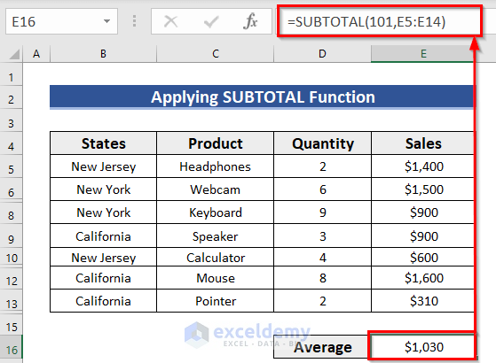
=SUBTOTAL(101,E5:E14)101 is the AVERAGE function and E5:E14 is the data range. The function will consider visible cells only, not the hidden ones.
- Press ENTER to see the result.
Read More: How to Average Only Visible Cells in Excel
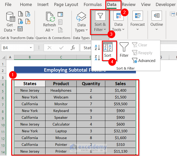
Method 3 – Using the Subtotal Feature to Find the Average in Excel
- Select data.
- Go the Data tab >> choose Sort & Filter >> select Sort.
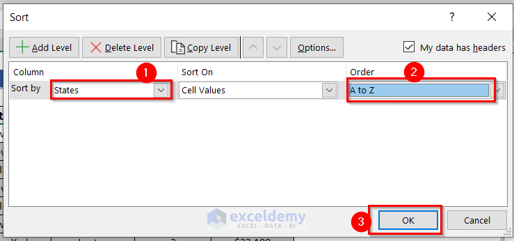
In the Sort dialog box:
- Choose States in Sort by and A to Z in Order.
- Click OK.
This is the output.
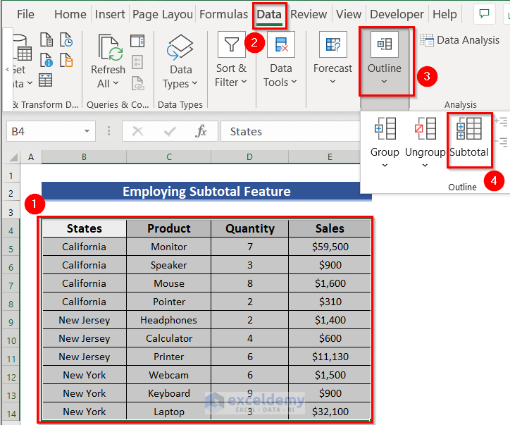
Use the Subtotal feature:
- Select data.
- Go to the Data tab >> choose Outline >> select Subtotal.
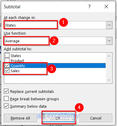
In the dialog box:
- Select States in At each change in the.
- Choose Average in Use function.
- Check Quantity and Sales.
- Click OK.
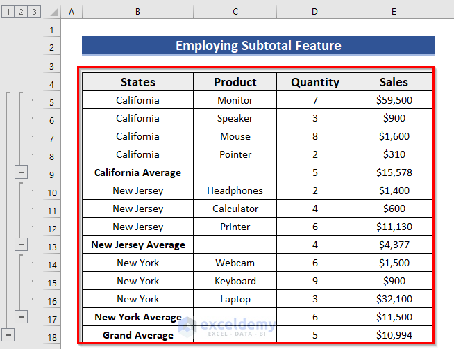
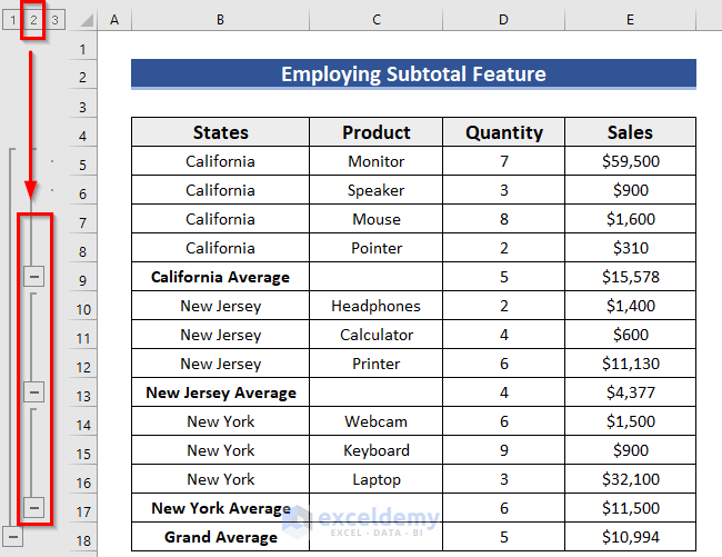
This is the output.
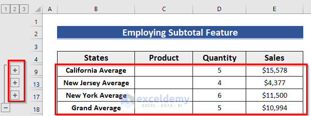
If you click the Minus (-) sign at the bottom of the 2nd box, you will see the average values. You can also click the 2nd box (on the left of the worksheet, beside the column name).
This is the output.
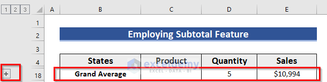
If you click the Minus (-) sign at the bottom of the 1st box, you will see the Grand Average values. You can also click the 1st box (on the left of the worksheet, beside the column name).
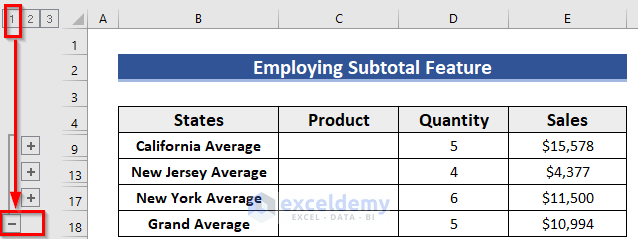
This is the output.
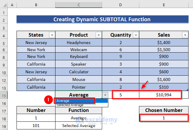
Method 4 – Creating a Dynamic SUBTOTAL Function to calculate the Average in Excel
Step 1: Inserting a Table to Create a Dynamic SUBTOTAL Function
- Select data.
- Press CTRL+T to create a table.
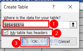
In Create Table:
- The table range is auto-selected.
- Check My table has headers.
- Click OK.
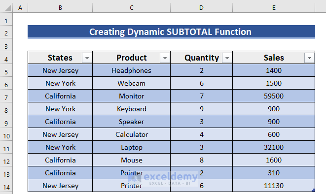
This is the output.
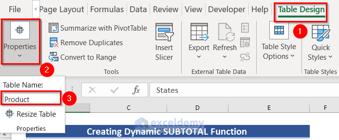
- Select any header.
- In Table Design >> go to Properties >> name your table. Here, Product.
Step 2: Using Functions to calculate the Subtotal Average
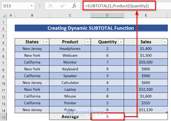
- Select a blank cell: D15 to keep the result.
- Enter the formula in D15 and press ENTER.
=SUBTOTAL(1,Product[Quantity])1 is the AVERAGE function, and Product[Quantity] is the data range: D5:D14. The function will consider all cells, even the hidden ones.
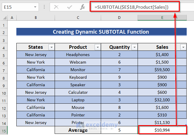
- Use the formula in E15 and press ENTER.
=SUBTOTAL(1,Product[Sales])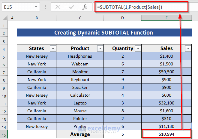
- Enter the function number and function name manually in B18:C19.
- Enter the following formula in E18 and press Enter.
=INDEX(B18:B19,MATCH(C15,C18:C19,0))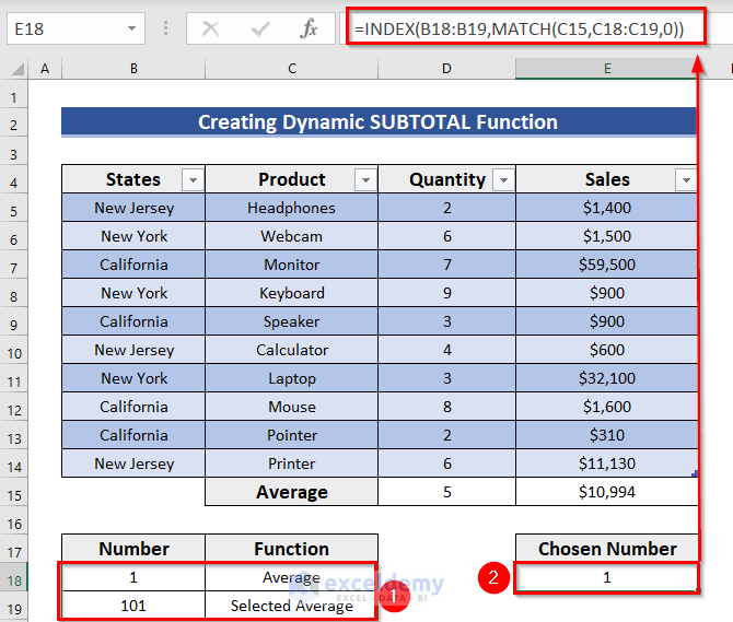
Formula Breakdown
- The MATCH function returns the position of the specified values.
- MATCH(C15,C18:C19,0)—> returns 1.
- The INDEX function returns a reference or value of the intersection of a given row and column.
- INDEX(B18:B19,1)—> returns 1.
- Use the formula below in D15.
=SUBTOTAL($E$18,Product[Quantity])E18 cell value was used instead of 1.
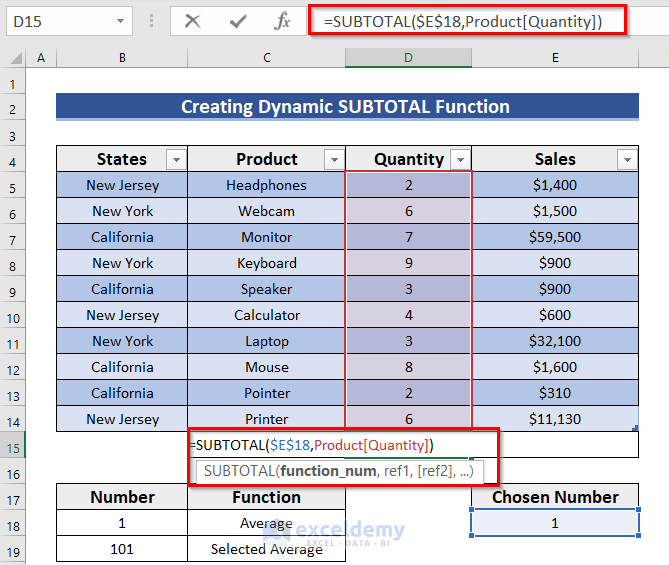
- Enter the formula in E15.
=SUBTOTAL($E$18,Product[Sales])E18 cell value was used instead of 1.
Step 3: Using the Data Validation Feature to Create a Dynamic SUBTOTAL Function
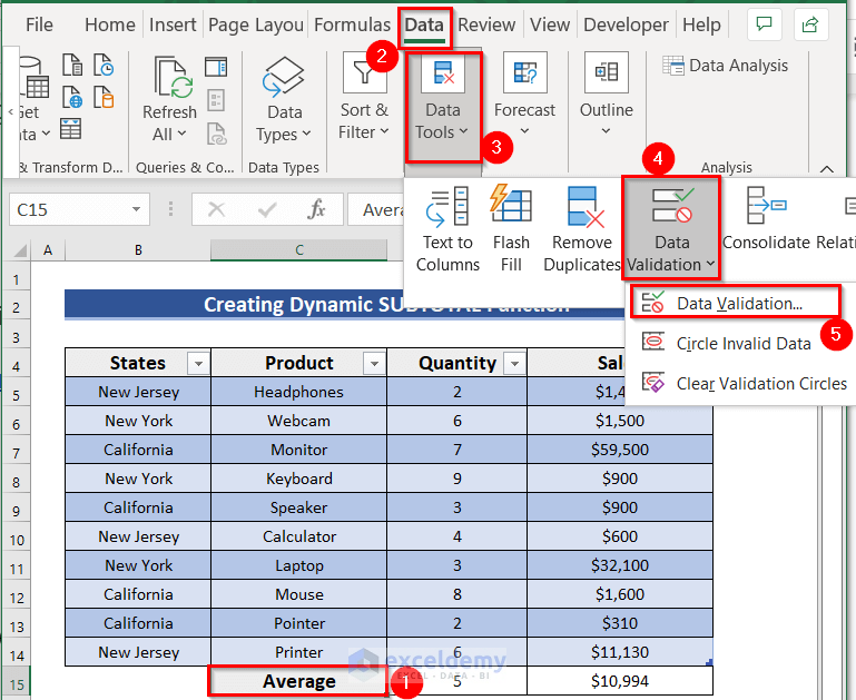
- Select C15 to insert the drop-down option.
- In Data >> go to Data Tools.
- In Data Validation >> choose Data Validation….
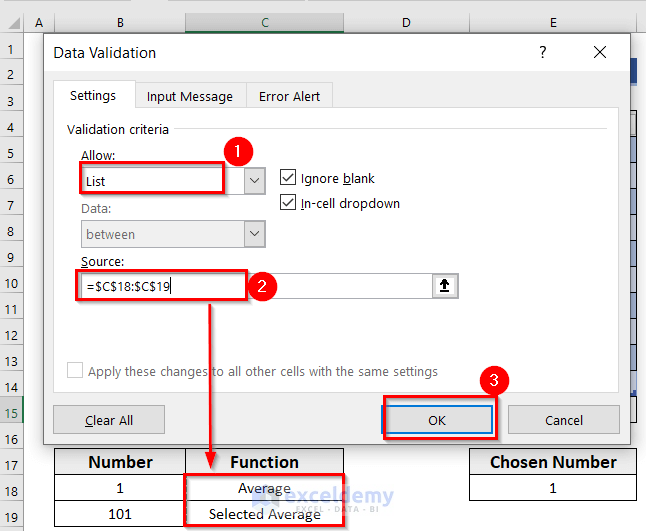
In the Data Validation dialog box:
- In Settings tab >> choose List in Allow:.
- Enter the Source and click OK.
Rows 7,11, and 14 were hidden.
When you choose Selected Average from the drop-down arrow, it will show the result ignoring the hidden cells.
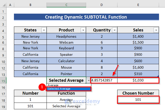
When you choose Average from the drop-down, it will show the result including the hidden cells.
Read More: How to Average Filtered Data in Excel
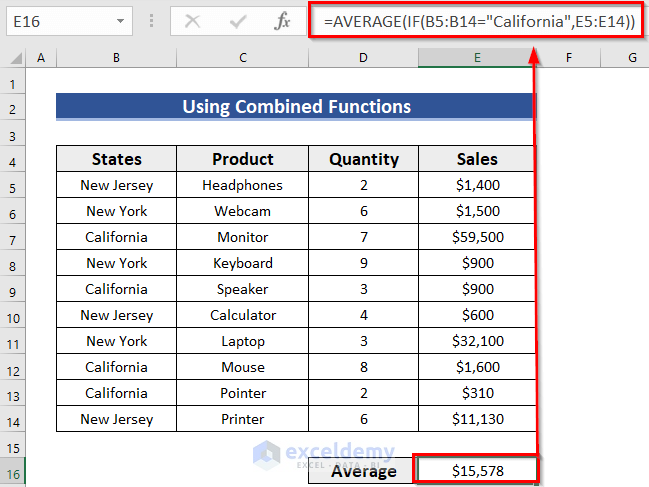
Method 5 – Using a Combination of Functions to Calculate the Subtotal Average
- Go to E16 and use the following formula.
=AVERAGE(IF(B5:B14="California",E5:E14))- Press ENTER to see the result.
You will see the average sales in California.
Formula Breakdown
The IF function returns the result that fulfills a given condition.
- B5:B14=”California” is a logical test. The function tests whether the cell value of the B column is California. Use the Inverted Comma in strings.
- E5:E14 if the logic is TRUE, it will return the cell value of column E. Otherwise, it returns FALSE.
- IF(B5:B14=”California”,E5:E14)—> returns {FALSE,FALSE,59500,FALSE,900,FALSE,FALSE,1600,310,FALSE}.
- The AVERAGE function finds the average of the above output.
- Output: 15,578
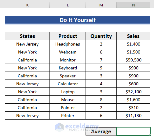
Practice Section
Practice here.
Download Practice Workbook
Download the practice workbook.
Related Articles
- How to Calculate Average and Standard Deviation in Excel
- How to Calculate Average Deviation in Excel Formula
- How to Calculate Average Excluding Outliers in Excel
- How to Calculate Average of Text in Excel
- How to Average Negative and Positive Numbers in Excel
<< Go Back to Calculate Average in Excel | How to Calculate in Excel | Learn Excel
Get FREE Advanced Excel Exercises with Solutions!
