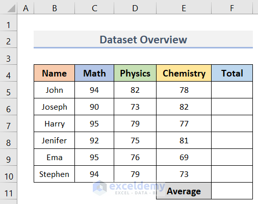
The dataset contains the names of some students and their marks in Math, Physics, and Chemistry. We will calculate each student’s total marks in all subjects in the range F5:F10 and calculate the average of the total marks in cell F11.
Method 1 – Inserting SUM & AVERAGE Formulas with AutoSum Tool in Excel
Steps:
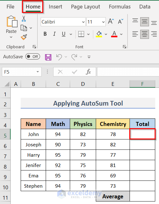
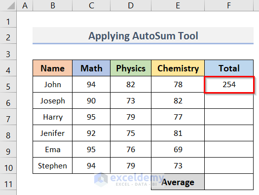
- Calculate the Total marks of the first student (John) in the three subjects.
- Activate cell F5 and go to the Home tab.
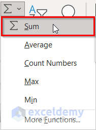
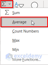
- Click on the AutoSum drop-down in the Editing group.

- To calculate the Total marks, select Sum from the drop-down menu.
- The SUM function with the range C5:E5 will be inserted automatically in the selected cell (F5).
- We will see the following formula in cell F5.
=SUM(C5:E5)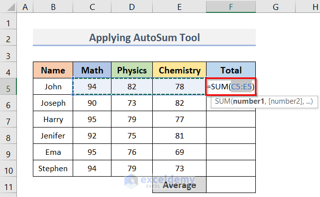
- Press Enter and get the Total marks of John in cell F5.
- To get the Total marks of the other students, put your cursor in the bottom-right corner of cell F5.
- You will see a plus sign (+) called the Fill Handle.
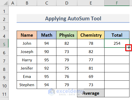
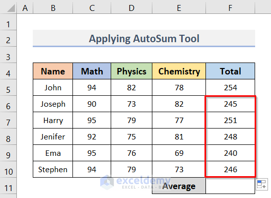
- Drag the Fill Handle to autofill the rest of the cells in the range F6:F10.
See the picture below.
- We can sum up the marks of the students.
- We will calculate the Average marks for all the students.
- Select cell F11 > go to the Home tab.
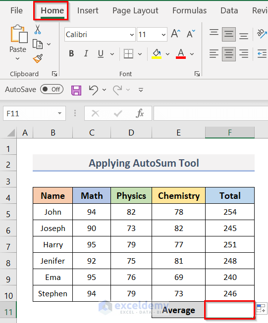
- Click on Average from the AutoSum dropdown menu.
- You will get the formula below in cell F11.
=AVERAGE(F5:F10)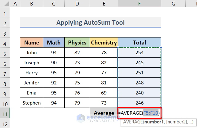
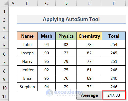
- Press Enter.
See the average value in cell F11 of the screenshot below.
Method 2 – Calculating Sum & Average in Excel with SUM & AVERAGE Functions
2.1 Inserting Range Reference
Steps:
- Go to cell F5 and type
"=".
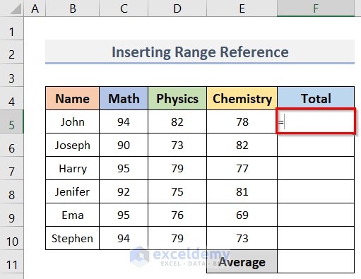
- To calculate the total marks of John type SUM, you will see the option SUM below the cell.
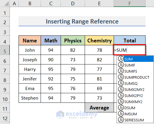
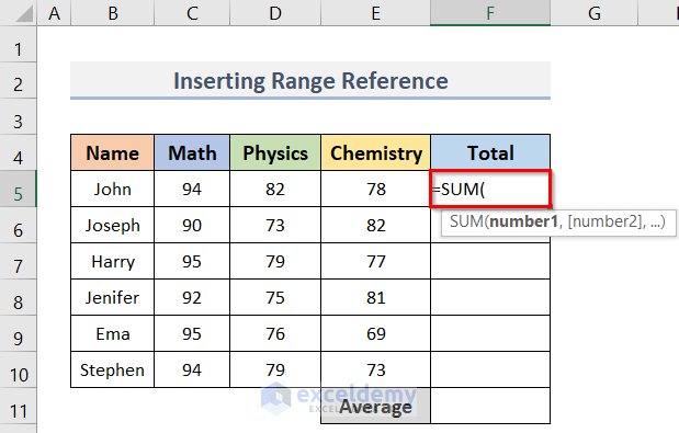
- Double-click on the SUM option.
- The SUM function will be inserted in the cell.
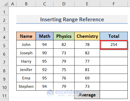
- Select the range C5:E5.
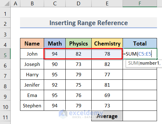
- Close the parenthesis.
- The final formula will be:
=SUM(C5:E5)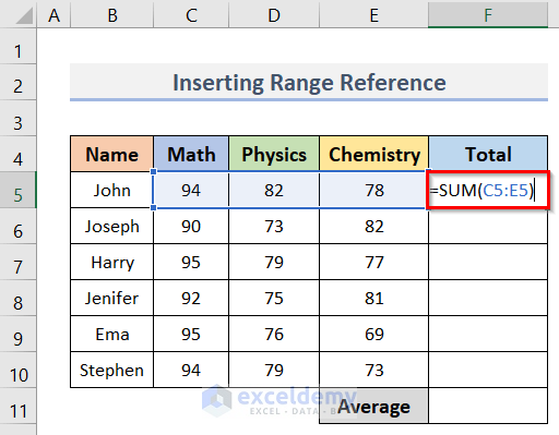
- Press the Enter key.
- You can calculate the total marks of John.
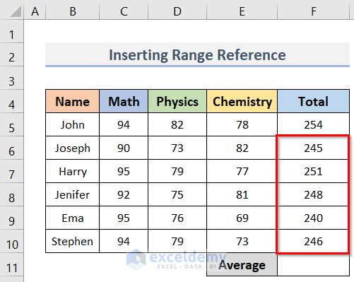
- Drag the Fill Handle to Autofill the cells for the rest of the students (F6:F10).
- We can determine the average marks of all the students in the class.
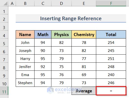
- Go to cell F11 > type
"=".
- Type AVERAGE and double-click on the AVERAGE option.
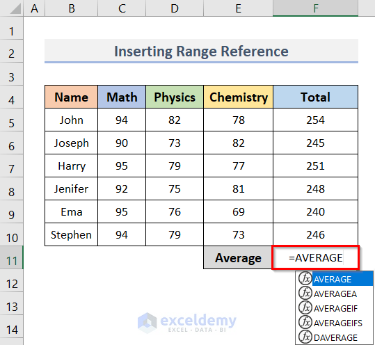
- Select the range F5:F10.
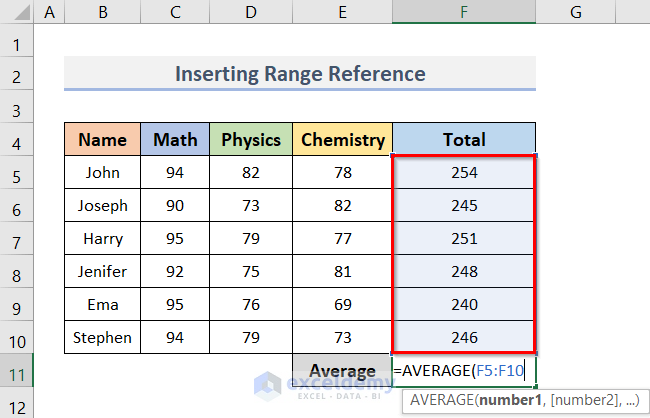
- Close the bracket.
- The final look of the formula will be:
=AVERAGE(F5:F10)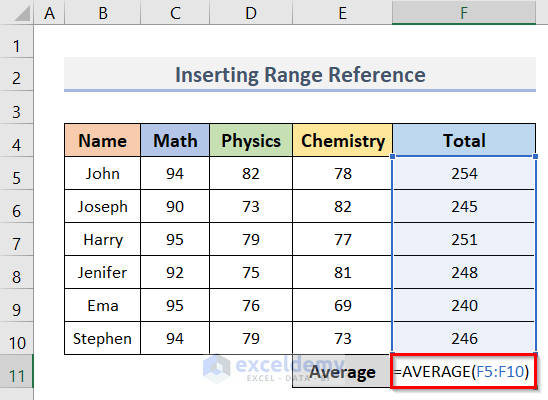
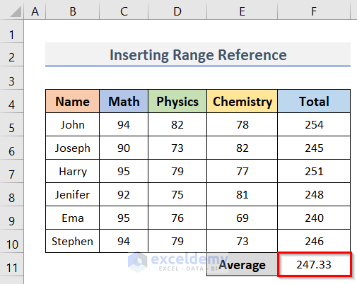
- Press Enter to find the output.
Read More: How to Calculate Average of Multiple Ranges in Excel
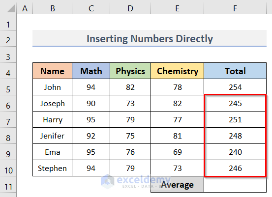
2.2 Enter Numbers Directly
Steps:
- Select cell F5.
- To get the total mark of John, enter the following formula:
=SUM(94,82,78)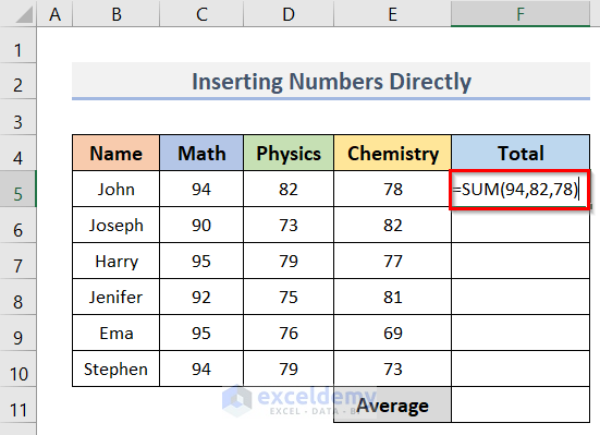
In this formula, we typed marks of John in Math, Physics, and Chemistry manually.
- After pressing Enter, we will get the total mark of John.
- Drag the plus sign to Autofill the range F6:F10.
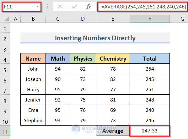
- To calculate the average mark, enter the formula below in cell F11:
=AVERAGE(254,245,251,248,240,246)- Lastly, press the Enter key.
Read More: How to Average Negative and Positive Numbers in Excel
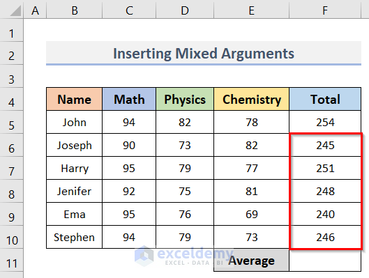
2.3 With Mixed Arguments
Steps:
- Select cell F5.
- Enter the following formula to get the total marks of the first student in all subjects.
=SUM(C5,D5,78)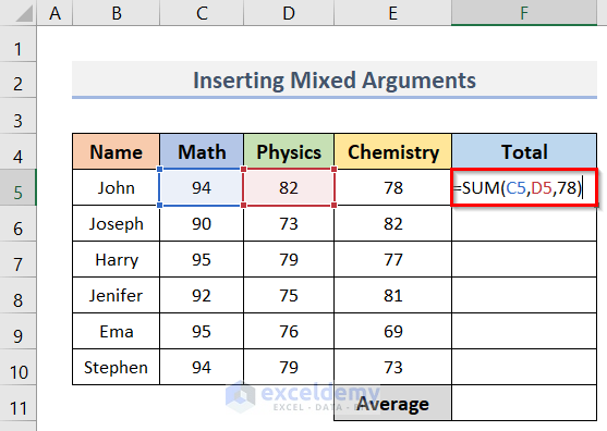
In the formula, C5 & D5 are the cell references, whereas 78 is a number.
- Press Enter to find the result in cell F5.
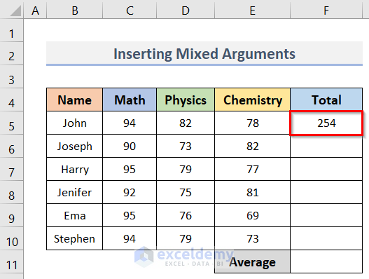
- Drag the plus sign to Autofill the rest of the cells of range F6:F10.
- To get the average marks of the students, enter the following formula in cell F11:
=AVERAGE(F5,F6,251,F8,F9,F10)- Press Enter to get the result.
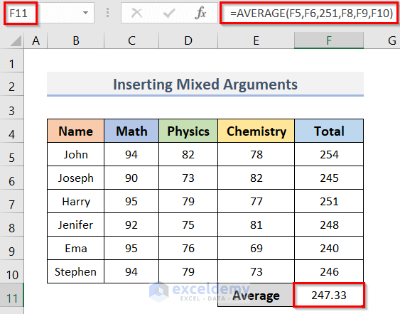
In this formula, F5, F6, F8, F9 and F10 are cell references. Besides, 251 is a number. So, we can see that the SUM and the AVERAGE functions support mixed arguments.
Read More: How to Average Filtered Data in Excel
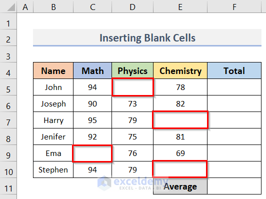
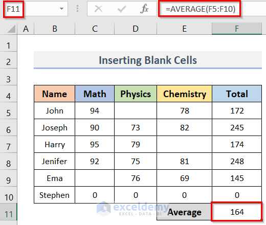
2.4 For Blank Cells and Zero Values
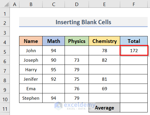
In the dataset below, D5, E7, C9, and E10 are blank cells. We will insert these cells along with the cells with numbers to calculate the students’ total and average marks.
Steps:
- Select cell F5.
- To calculate the total marks of John, type the formula below:
=SUM(C5:E5)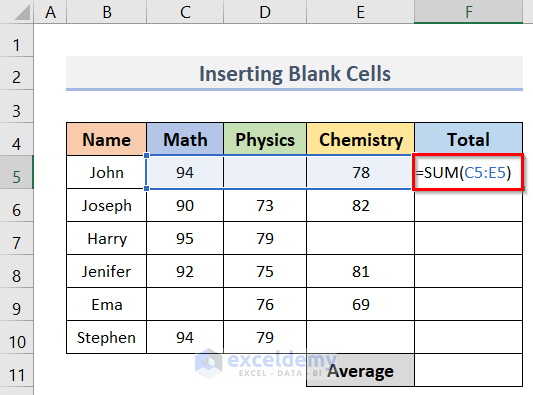
- Press Enter to get the result.
- The SUM formula ignores the blank cell (D5) and adds the rest of the cells (C5, E5).
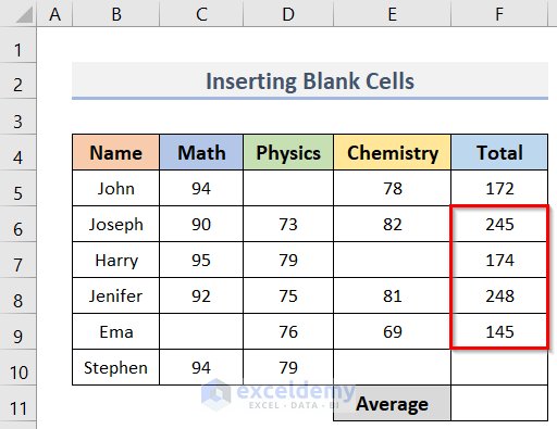
- Calculate the total marks for other students by dragging the Fill Handle.
- To calculate the average marks of the students in the range F5:F10.
- Enter the formula below in cell F11:
=AVERAGE(F5:F10)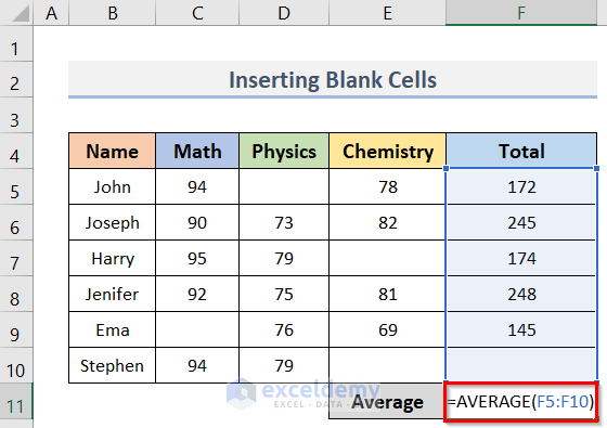
The cell F10 in the formula is blank.
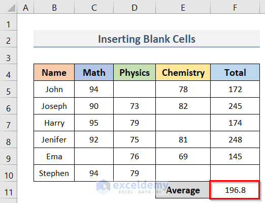
- Press Enter to get the average mark in cell F11.
- The AVERAGE formula ignored the blank cell (F10) and calculated the average for the cells containing numbers (F5:F9).
- If cell F10 contains a zero value (0) then we get the result like the picture below.
- The AVERAGE formula included the cell (F10) with zero value in the calculation.
Read More: How to Calculate Average in Excel Excluding 0
2.5 SUM Function with AVERAGE Function
Steps:
- Calculate the total marks using the SUM function like the previous one.
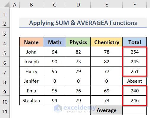
- If we use the AVERAGE function to calculate the average marks, we will see that this function does not consider the text string in the calculation.
- However, it ignores the text string and calculates the average for the cells containing numbers.
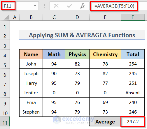
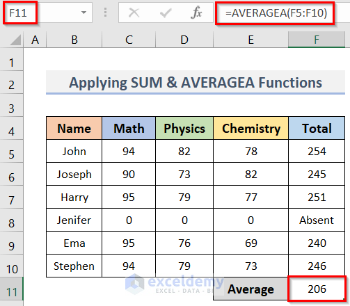
- To include the text string in calculating the average, we can use the AVERAGE function.
- Enter the following formula in cell F11:
=AVERAGEA(F5:F10)- Press Enter.
- The result is in cell F11 of the picture below..
Read More: How to Do Subtotal Average in Excel
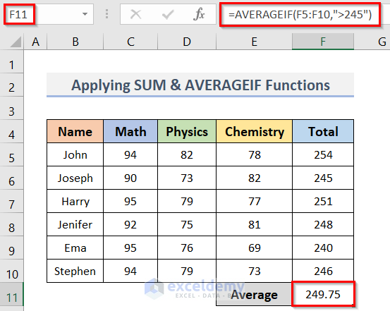
2.6 Combine SUM & AVERAGEIF Functions
Steps:
- Calculate the total marks (F5:F10) using the SUM function (described in the previous methods).
- Enter the formula below in cell F11 to calculate the average of the total marks greater than 245:
=AVERAGEIF(F5:F10,">245")- Press Enter to get the result in cell F11 of the image below.
2.7 SUM Function with AVERAGEIFS Function
Steps:
- Use the SUM function to calculate the total marks (F5:F10) like the previous methods.
- Calculate the average marks of the students by entering the following formula in cell F11:
=AVERAGEIFS(F5:F10,B5:B10,"*e*",E5:E10,">70")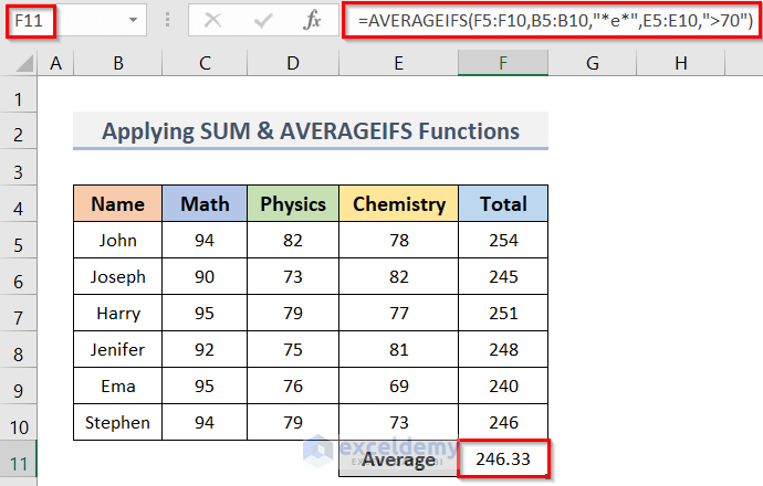
This formula calculates the average of the total marks (F5:F10) for the students whose names (B5:B10) contain the letter "e" and whose marks in Chemistry (E5:E10) are greater than 70. In this formula, we used the wildcard (*) to denote the letter "e".
Method 3 – Using an Array Formula to Find Sum & Average in Excel
Steps:
- Calculate the total marks (F5:F10) using the SUM function like before.
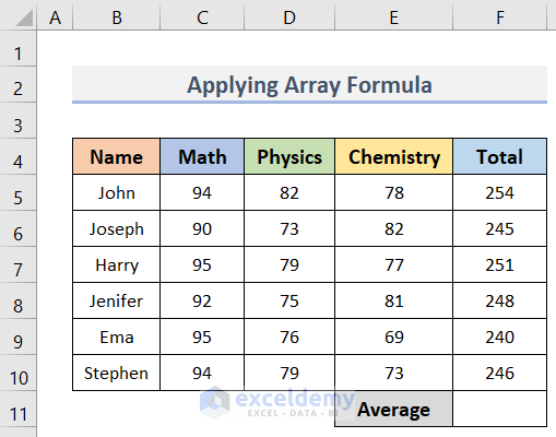
- Go to cell F11.
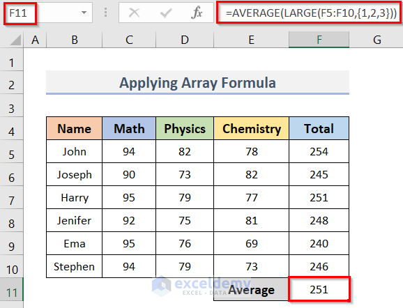
- To determine the average of the three largest marks (Total), enter the following formula in cell F11:
=AVERAGE(LARGE(F5:F10,{1,2,3}))- Press Ctrl + Shift + Enter to terminate the array formula.
- You will get the desired average in cell F11 like the picture below.
How Does the Formula Work?
- LARGE(F5:F10,{1,2,3}): Returns the three largest numbers from the F5:F10 range.
- AVERAGE(LARGE(F5:F10,{1,2,3})): Returns the average of the three largest numbers.
Download Practice Workbook
Download the practice workbook from here.
Related Articles
- How to Calculate Average and Standard Deviation in Excel
- How to Calculate Average Deviation in Excel Formula
- How to Calculate Average Excluding Outliers in Excel
<< Go Back to Calculate Average in Excel | How to Calculate in Excel | Learn Excel
Get FREE Advanced Excel Exercises with Solutions!
