Method 1 – Calculate Average of Multiple Columns Using AVERAGE Function
Steps:
- Type the below formula in cell B13 to calculate the average of ranges B5:B10, C5:D9, and E6:E11.
=AVERAGE(B5:B10,C5:D9,E6:E11)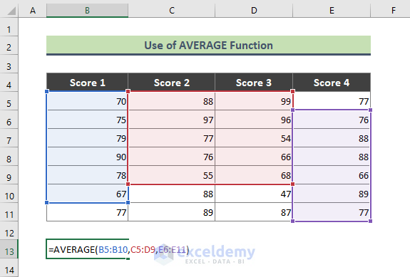
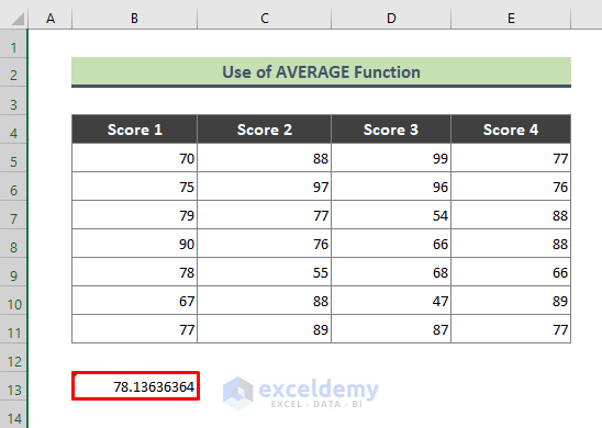
- Hit Enter, and you will get the average of the specified ranges of columns B, C, D, and E.
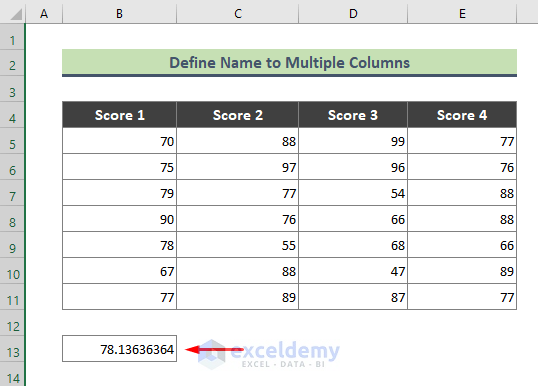
Method 2 – Define a Name to Multiple Columns and Then Get the Average
Steps:
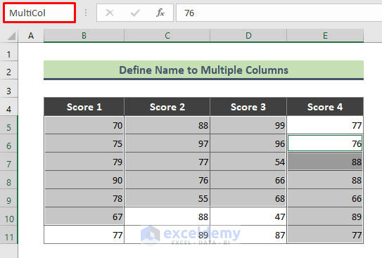
- Select the expected ranges from multiple columns by pressing the Ctrl key.
- Go to the Name Box, give a name, and press Enter. We named the below ranges as MultiCol.
- Type the below formula in cell B13 and hit Enter.
=AVERAGE(MultiCol)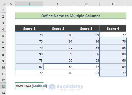
- Here is the ultimate average you will get.
Method 3 – Excel AVERAGEIF Function to Calculate Average of Multiple Columns
3.1. Get Average of Cells that Match a Criteria Exactly
We have a dataset (B4:C12) containing several fruit names and their qualities in columns B and C. Look for particular fruit names (here, Apple) in column B and calculate their average from column C.

Steps:
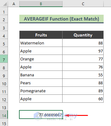
- Type the following formula in cell C14 and hit Enter.
=AVERAGEIF(B5:B12,"Apple",C5:C12)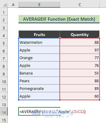
- I will get the average of the quantities of all apples on this dataset.
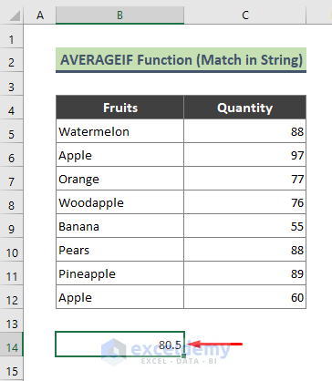
3.2. Calculate Average of Cells that Match Criteria in a String
Steps:
- Type the below formula in cell C14.
=AVERAGEIF(B5:B12,"*Apple*",C5:C12)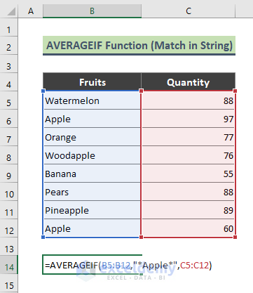
- Press Enter and get the below result.
Method 4 – Combination of AVERAGEIF and SUMIF Functions to Get an Average of Multiple Columns
Steps:
- Type the below formula in cell E13 and hit Enter.
=AVERAGEIF($B$5:$B$10,B13,$E$5:$E$10)*SUMIF($B$5:$B$10,B13,$C$5:$C$10)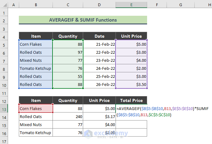
- Get the below result. Use the Fill Handle (+) tool to copy the formula to the rest of the cells.
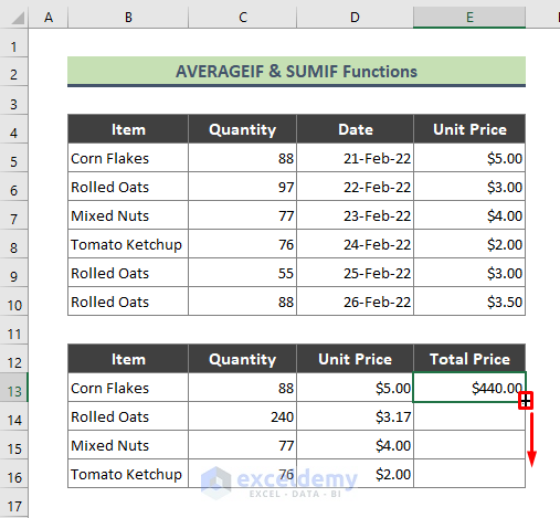
- Get the total price for all the items as below.
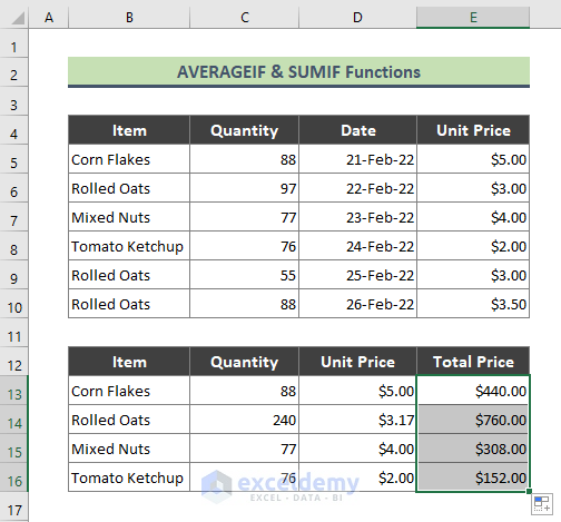
How Does the Formula Work?
➤ AVERAGEIF($B$5:$B$10,B13,$E$5:$E$10)
This part of the formula returns the Unit Price of the cell content of cell B13 (Corn Flakes) which is: {5}
➤ SUMIF($B$5:$B$10,B13,$C$5:$C$10)
This part of the formula returns the sold Quantity of Corn Flakes, which is: {88}
➤ AVERAGEIF($B$5:$B$10,B13,$E$5:$E$10)*SUMIF($B$5:$B$10,B13,$C$5:$C$10)
The above formula multiplies 5 by 88 and returns: {440}
Method 5 – Combination of Excel AVERAGE and LARGE Functions to Get Average from Multiple Columns
Steps:
- Type the below formula in cell B13 and press Enter.
=AVERAGE(LARGE(B11:E11, {1,2,3}))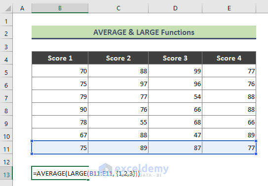
- Get the average of the top 3 values from the range B11:E11 spread over multiple columns.
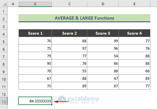
The LARGE function returns the 3 largest values (89, 87, & 77) in the range B11:E11. Later, the AVERAGE function returns the average of the above 3 numbers.
⏩ Note:
You can use the SMALL function along with the AVERAGE function to calculate the average of the most minor numbers in a range spread over multiple columns.
Method 6 – Excel OFFSET, AVERAGE, and COUNT Functions to Calculate the Average of Last N Values in Multiple Columns
Steps:
- Type the following formula in cell B13 and hit Enter.
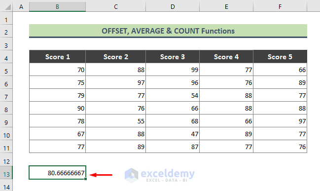
=AVERAGE(OFFSET(B5,0,COUNT(B5:F5)-3,1,3))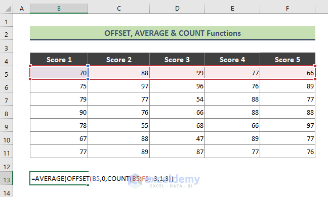
- Get below average.
How Does the Formula Work?
➤ COUNT(B5:F5)
This part of the formula returns: {5}
➤ (OFFSET(B5,0,COUNT(B5:F5)-3,1,3)
This part of the formula returns the last 3 values of the range B5:F5: {99,77,66}
➤ AVERAGE(OFFSET(B5,0,COUNT(B5:F5)-3,1,3))
The formula returns the average of the last 3 values (99,77,66) which is: {80.66666667}
Download Practice Workbook
You can download the practice workbook that we have used to prepare this article.
Related Articles
- How to Exclude a Cell in Excel AVERAGE Formula
- How to Find Average of Specific Cells in Excel
- How to Average Only Visible Cells in Excel
- How to Find Average with Blank Cells in Excel
- How to Fix Divide by Zero Error for Average Calculation in Excel
- How to Ignore #N/A Error When Getting Average in Excel
- [Fixed!] AVERAGE Formula Not Working in Excel
<< Go Back to Calculate Average in Excel | How to Calculate in Excel | Learn Excel
Get FREE Advanced Excel Exercises with Solutions!
