Method 1 – Input Argument Manually to Exclude a Cell in Excel AVERAGE Formula
In the sample dataset, we have Sales Amounts for different persons on different days of the week. We can see there are zero and blank cells in the dataset. If we input range B5:E15 as the argument of the AVERAGE function it will calculate the average considering the zero and blank cells. But we want to exclude zero and blank cells from the calculation of the average.
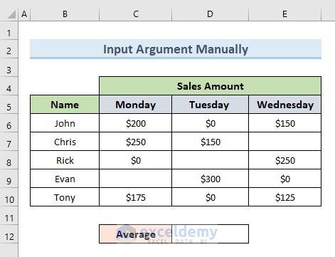
STEPS:
- Select cell D12 where we want to return the average value.
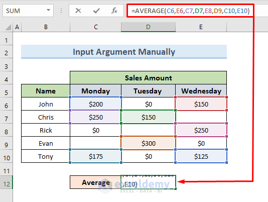
- Insert the following formula in that cell.
=AVERAGE(C6,E6,C7,D7,E8,D9,C10,E10)- To exclude the zero and blank cells hold the Ctrl key and select the cells that you want to take as arguments in the formula.
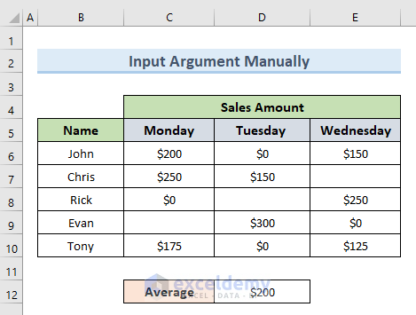
- Press Enter.
- It gives output of the average value only for selected cells in cell D12.
Method 2 – Ignore Blank/Zero Cells to Exclude a Cell in Excel AVERAGE Formula
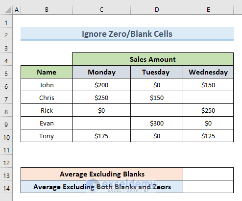
STEPS:
- Select cell D13.
- Insert the following formula in that cell.
=AVERAGE(C6:E10)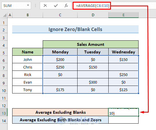
- Press Enter.
It gives the average value for the range C6:E10.
- Go to the File tab.

- Select Options.

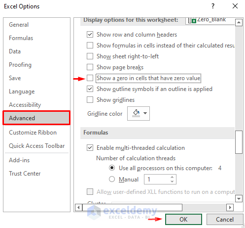
- Select the option Advanced from the newly appeared dialogue box.
- Scroll down and uncheck the option Show a zero in cells that have zero value from the section Display options for this worksheet.
- Press OK.
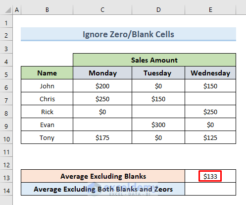
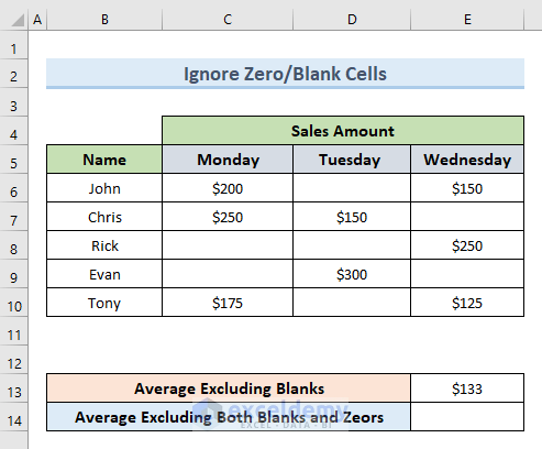
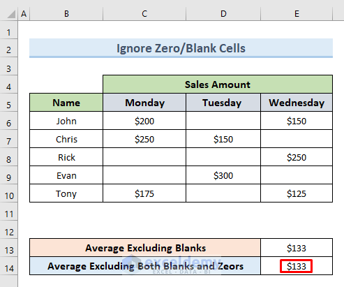
- This will remove the zero values from the dataset.
- Select cell E14 and insert the following formula in that cell.
=AVERAGE(C6:E10)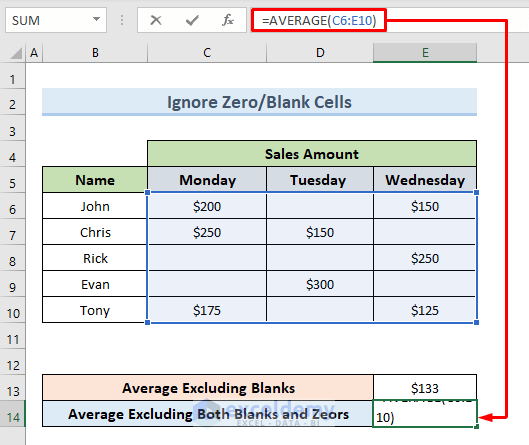
- Press Enter.
- The result is the same for both cases. So, if we have zero values in the dataset, we have to delete them manually to exclude them from the calculation of the AVERAGE formula.
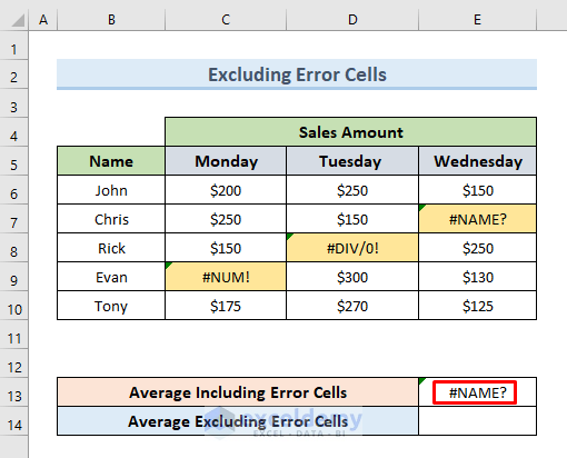
Method 3 – Use AVERAGE Formula for Ignoring Error Cells
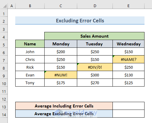
STEPS:
- Select cell D13 and insert the following formula.
=AVERAGE(C6:E10)- Press Enter.
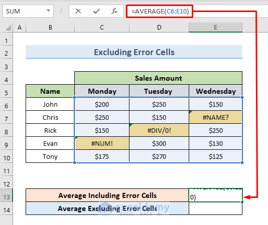
- The command returns an error in cell D13.
- Select cell D14 and insert the following formula.
=AVERAGE(IFERROR(C6:E10,""))- Press Enter.
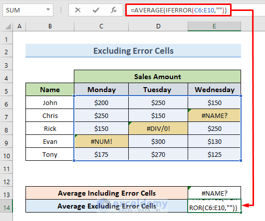
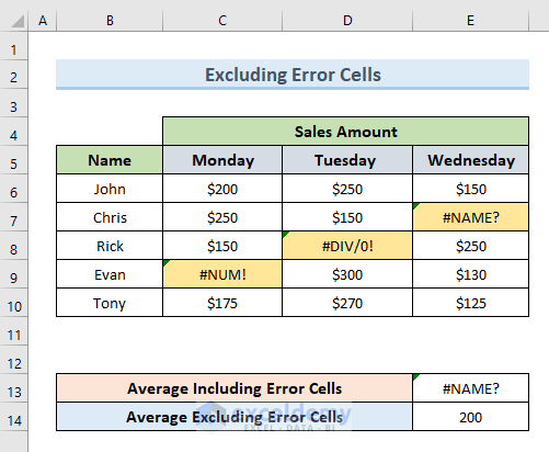
- The error cells will now be ignored. We will get the average value excluding error cells in cell D14.
How Does the Formula Work?
- IFERROR(C6:E10,””): This part checks if there are any error values in the data range C6:C10 and returns values excluding error cells.
- AVERAGE(IFERROR(C6:E10,””)): Returns the average value for the cells in the data range C6:C10 excluding error cells.
Read More: How to Ignore #N/A Error When Getting Average in Excel
Method 4 – Combination of Excel SUM and COUNT Functions to Exclude Cells
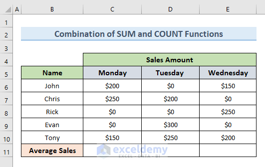
STEPS:
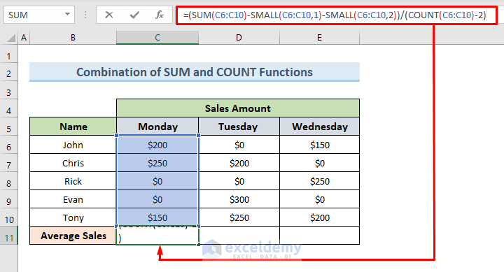
- Select cell C11 and insert the following formula.
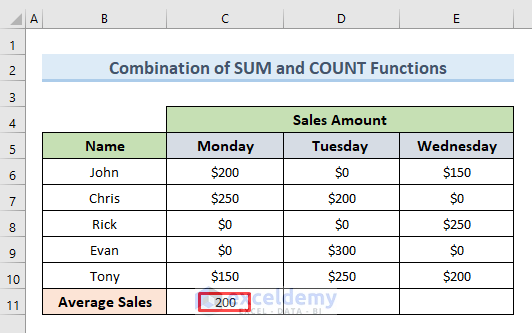
=(SUM(C6:C10)-SMALL(C6:C10,1)-SMALL(C6:C10,2))/(COUNT(C6:C10)-2)- Press Enter.
- The command returns the average value on Monday in cell C13. We have excluded the zero cells from our calculation.
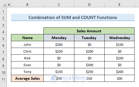
- Select cell C13 and drag the Fill Handle tool horizontally to cell E11.
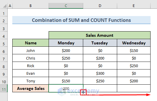
- The above action will copy the formula of cell C13 in cells D13 & E13 and return the average Sales Amounts for Tuesday and Wednesday.
How Does the Formula Work?
- COUNT(C6:C10)-2): Counts total cell numbers from C6 to C10 and ignores the lowest two cells which are zero cells.
- SUM(C6:C10): Returns the totals for cells C6 to C10.
- SUM(C6:C10)-SMALL(C6:C10,1)-SMALL(C6:C10,2): Here the SMALL function determines the lowest two parts of the range C6:C10. Then the lowest two values are subtracted from the total.
- SUM(C6:C10)-SMALL(C6:C10,1)-SMALL(C6:C10,2))/(COUNT(C6:C10)-2: Returns the average excluding two zero cells.
Download Practice Workbook
Related Articles
- How to Average a Column in Excel
- How to Calculate Average of Multiple Columns in Excel
- How to Average Every Nth Row in Excel
- How to Calculate Average of Multiple Ranges in Excel
- How to Average Only Visible Cells in Excel
- How to Find Average of Specific Cells in Excel
- How to Fix Divide by Zero Error for Average Calculation in Excel
- [Fixed!] AVERAGE Formula Not Working in Excel
<< Go Back to Conditional Average | Calculate Average | How to Calculate in Excel | Learn Excel
Get FREE Advanced Excel Exercises with Solutions!
