[Fixed!] AVERAGE Formula Not Working in Excel (6 Solutions)

You may face some problems in some cases while using the AVERAGE formula in Excel. But no worries, there are a lot of ways to solve it. This article will provide you with the 6 best methods to overcome the situation when the AVERAGE formula is not working properly in Excel.

AVERAGE Formula Not Working in Excel: 6 Solutions

To explore the methods we’ll use the following dataset that represents some salespersons’ sales in different regions.

1. Remove Blank Space When the Average Formula Is Not Working in Excel

If the formula based on the AVERAGE function doesn’t give you the correct result then there may be blank spaces within the values. The AVERAGE formula then skips that value and gives an answer without counting it.

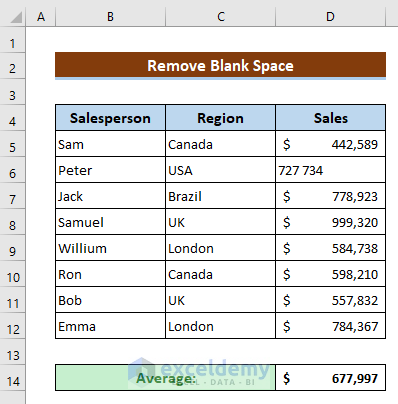
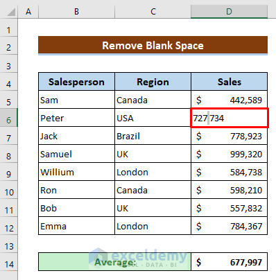
Please have a look that we have a blank space in the second sale.

To fix it, just remove the blank space and hit Enter.

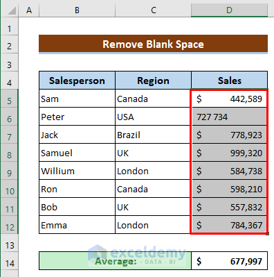
If you have a large dataset then you can use the Find and Replace tool to find and remove the spaces.

Select the data range D5:D12.

Press Ctrl+H to open the Find and Replace tool.
Type space in the Find what box and keep the Replace with box empty.
Finally, press Replace All.

A message box will show the result.

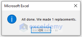
And then you will get an accurate result.

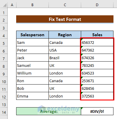
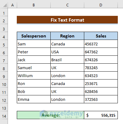
2. Change Text to Numeric Format If the Average Formula Does Not Work

Another common reason is that maybe you have inputted the numbers in text format. So the AVERAGE formula gives you #DIV/0! error.
A triangle-shaped green sign located in the top-left corner of the cells will give you the message that you have used the wrong format.

If you change the format from the Home tab then it won’t work. To solve it, select the cells and click on the error sign.
Later, click Convert to Number from the Context Menu.

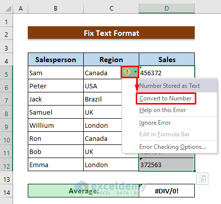
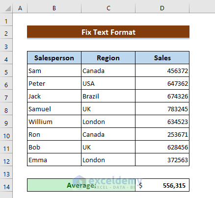
Then you will get the average accurately.

Also, you can use the Text to Columns command to do it.

Select the data range D5:D12.
Then click as follows: Data > Text to Columns.
Soon after a dialog box will open up.

Nothing to do here, press Next.

Again press Next.

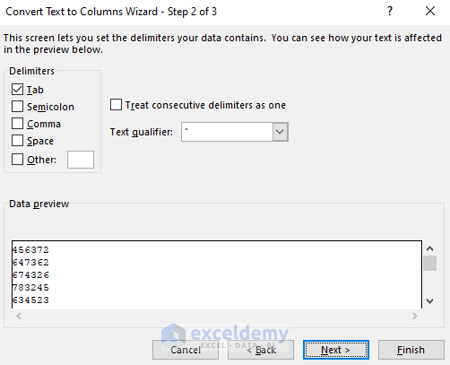
Mark General and finally, just press Finish.

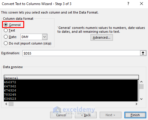
Now the AVERAGE formula is working properly.

3. Remove the Text in the Dataset

If your dataset has non-numeric values, the AVERAGE formula will skip those values. Have a look at the dataset, Samuel has no sales so if we find an average then the AVERAGE formula won’t count that value. That’s why you won’t get the proper answer.

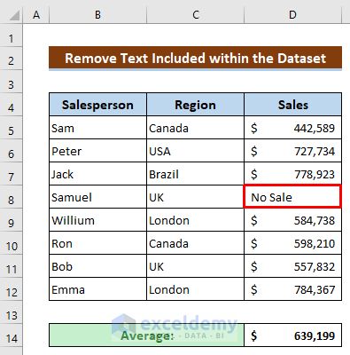
The solution is to type 0 instead of the text No Sale and then the AVERAGE formula will count it.

Here’s the output including zero.

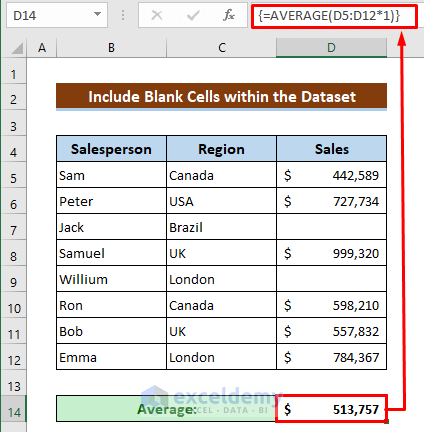
4. Array Formula for Blank Cells in the Dataset

The AVERAGE function skips blank cells but to calculate the average you must have to count every cell.

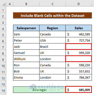
To solve the problem apply the following formula in cell D14.

=AVERAGE(D5:D12*1)

Finally, press Ctrl+Shift+Enter and you will get the correct answer.

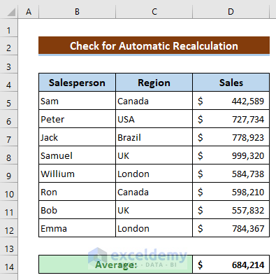
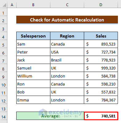
5. Check for Automatic Calculation If the Average Formula Is Not Working in Excel

Excel has some options for calculating operations. If you do not activate the Automatic option and change any value, Excel will not recalculate the average.

Look at the following dataset. Here the average value is correct.

Now let’s change a value. I have changed the first sales and see that there is no change in the calculated average.

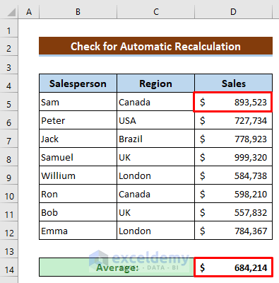
Because I kept Manual mode in Calculation Options from the Formulas tab.

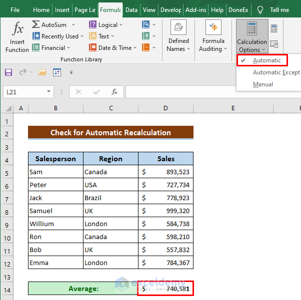
To check it, click as follows: Formulas > Calculation Options.

Keep it Automatic, then it will recalculate every time for any change.

If you don’t want to turn on Automatic mode then press Calculate Now from the Calculation section or use the F9 key to recalculate for the whole workbook.
Press the Calculate Sheet from the Calculation section or use the Shift+F9 key to recalculate for the active sheet.

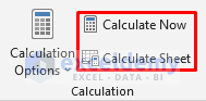
Output after pressing Calculate Sheet, the average is changed now.

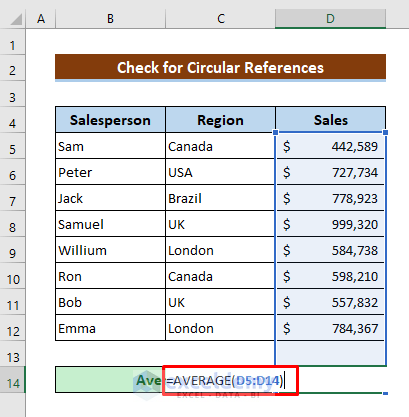
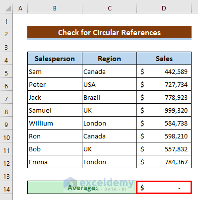
6. Check for Circular References When the Average Formula in Excel Is Not Working

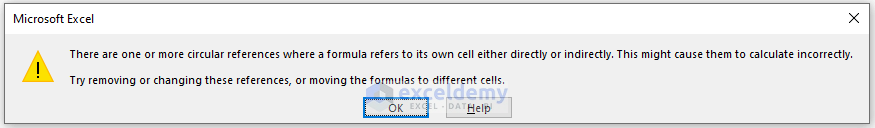
If you use a Circular Reference in your formula then again you won’t get the correct result for calculating the average. Have a look at the following dataset that I have used cell D14 in my formula which is the cell where I am writing the formula. If I press Enter then let’s see what is gonna happen.

You will get this type of message mentioning that you have used a Circular Reference. Press OK there.

Soon after you will get the output like this.

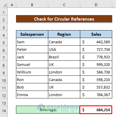
Give proper cell reference D5:D12 to overcome this problem.

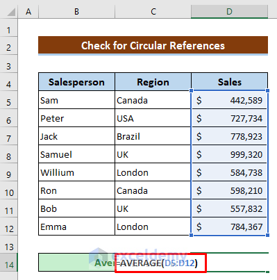
The problem is solved now.

Find Average Ignoring Errors in Excel

When you are working in a large dataset, using values from other sheets or cell references then it’s quite possible to remain error in values. And then the AVERAGE formula will show an error too.

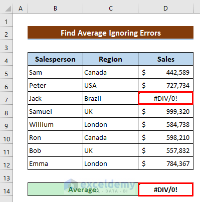
But you can easily count average ignoring those errors in Excel. You can do it in 2 ways.

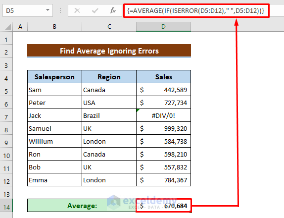
1. Use AVERAGE, IF, and ISERROR Functions

Combine the AVERAGE, IF, and ISERROR functions to calculate the average ignoring errors.

Type the following formula in cell D14.

=AVERAGE(IF(ISERROR(D5:D12)," ",D5:D12))

Finally, just hit the Ctrl+Shift+Enter button, because it’s an array formula.

⏬ Formula Breakdown:

➥ ISERROR(D5:D12)
The ISERROR function will check whether there is any error or not in the range D5:D12. It will return as {FALSE;FALSE;TRUE;FALSE;FALSE;FALSE;FALSE;FALSE}

➥ IF(ISERROR(D5:D12),” “,D5:D12)
The IF function will replace TRUE by space and FALSE by the corresponding value. So it returns- {442589;727734;” “;999320;584738;598210;557832;784367}

➥ AVERAGE(IF(ISERROR(D5:D12),” “,D5:D12))
Finally, the AVERAGE function will calculate the average for those values. For cell D5, it will return as- 670684

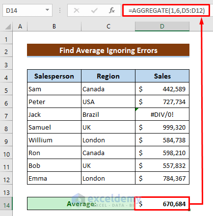
2. Apply AGGREGATE Function

Using the AGGREGATE function is the best way to do it rather than the previous way.

Type the following formula in cell D14.

=AGGREGATE(1,6,D5:D12)

Later, just press the Enter button to get the output.

Download Practice Workbook

You can download the free Excel template from here and practice on your own.

Average Formula Not Working.xlsx

Conclusion

I hope the procedures described above will be good enough to solve the problem when the average formula is not working in Excel. Feel free to ask any question in the comment section and please give me feedback.