If you’re looking for a way to avoid the divide-by-zero error during the average calculation in Excel, you’ve come to the right place. There are some methods for avoiding the divide-by-zero error in Excel’s average calculation. This article will walk you through each step with illustrations so you can easily apply them to your situation. Let us now move on to the meat of the article.
When #DIV/0! Error Occurs in Average Calculation?
While doing the average calculation of various types of datasets, you may find #DIV/0! error in the cell. This may happen for certain reasons.
- If you want to calculate the average of text values
Sometimes, you may insert an average formula for a range that may contain text values. If any text value comes into the average formula, it will return #DIV/0! error as an output. As a result, when selecting the range for the AVERAGE function, make sure that the cells do not contain text values.
- If the numbers are in TEXT format
You can find any Excel file where the numbers have been converted to TEXT format. In this case, you can’t use the AVERAGE function to calculate the average of the numbers, and if you do, you’ll get #DIV/0! error.
In this section, I will demonstrate how to avoid the divide-by-zero error when calculating the average in Excel. In this article, you will find thorough explanations with illustrative examples for every topic. Here, I have utilized the Microsoft 365 version. However, you may use any other version depending on your availability. Please leave a comment if any part of this article does not work in your version.
Case 1: Selection of a Wrong Range in AVERAGE Function Can Cause Divide by Zero Error for Average Calculation
It may happen sometimes when you have selected the wrong range of cells to calculate an average.
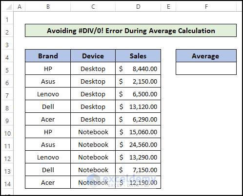
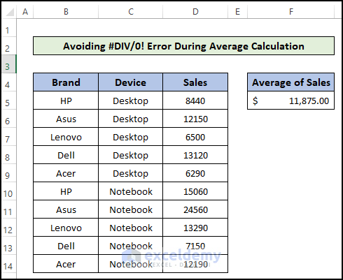
- Suppose, you want to calculate the average sales of all products as shown in the screenshot below. Here, I have an Excel worksheet containing sales data for some tech products.
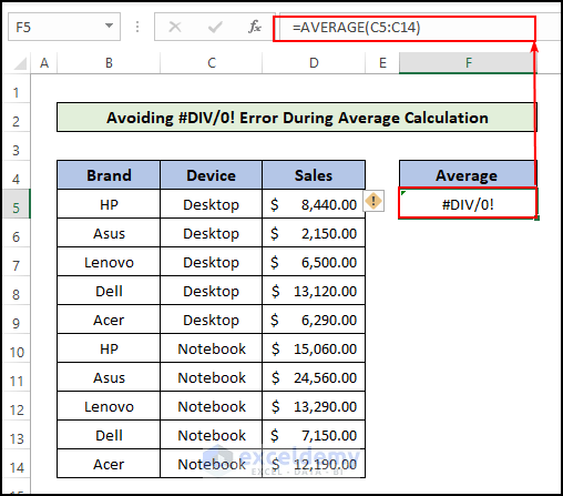
- To calculate the average sales, I should use the data range D5:D14 in the AVERAGE function. But I have used the range C5:C14. So, Excel has tried to calculate the average of device names which is impossible. So, it returns #DIV/0! error as an output.
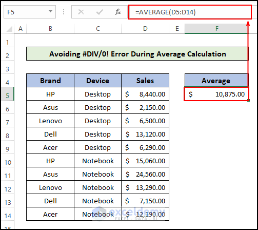
- Now, I have corrected the cell reference containing only numerical data and gives the average value of sales properly.
Read More: How to Ignore #N/A Error When Getting Average in Excel
Case 2: If Numbers Are in Text Format with Leading Apostrophes Then You Can Face Divide by Zero Error
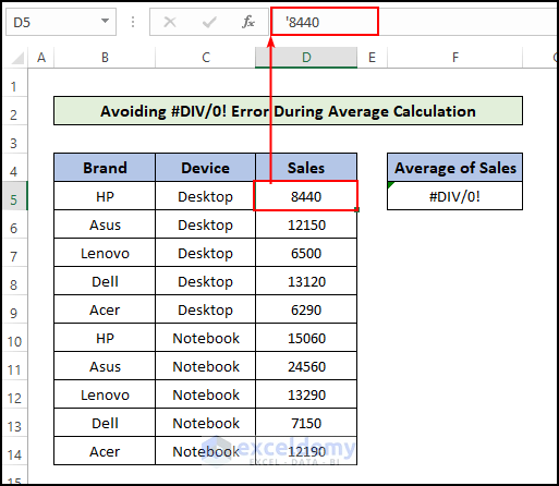
Let’s say a coworker gave you an Excel file with some sales information and you have assumed the sales values are in number format as usual. But, you are facing #DIV/0! error as an output while calculating the average of the sales values. And, you have double-checked that there isn’t any text value in the selected cell.
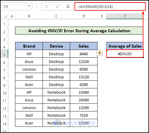
- This is happening because the previous user or the creator of the Excel file has converted the numbers to Text format by adding an apostrophe (`) in front of the numbers. So, you have to remove the apostrophe manually from each cell of the range to calculate the average. There is another way to remove the apostrophe from the front of numbers which is using the Text to Columns feature of Excel.
Solution: Remove Leading Apostrophe from Numbers with Text To Column Feature
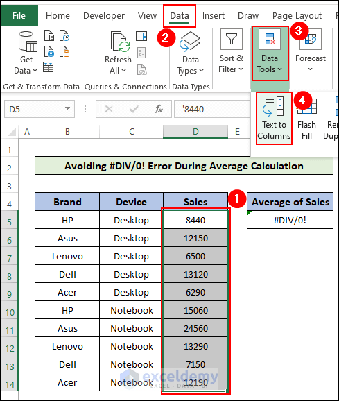
- For this, first, select the cells which contain apostrophes in front.
- Then, go to the Data tab in the top ribbon and select the Text to Columns feature in the Data Tools section.
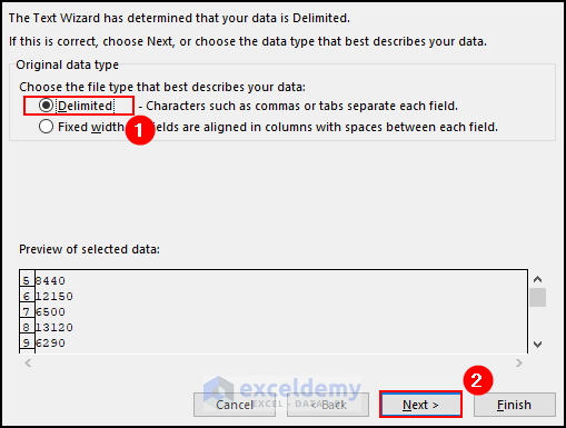
- Then, a new window will appear. Here, select the Delimited options and press Next after that.
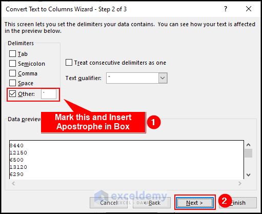
- In the 2nd step, you have to specify the delimiter which separates the text.
- Here, mark the Other checkbox under Delimiters and insert an apostrophe in the box.
- Then, press the Next button.
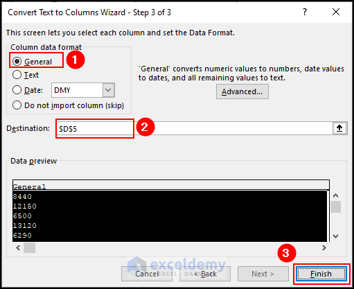
- In the third and last step, you can select General as the Column data format.
- Then, specify the first cell of the selected data range as the Destination.
- Finally, press the Finish button.
- As a result, you will see that, the #DIV/0! error vanishes and the average of the selected data range is shown in the box. Thus, you have removed the #DIV/0! error and calculated the average of a data range in Excel.
Download Practice Workbook
You can download the practice workbook here:
Conclusion
In this article, you have found how to avoid the divide by zero error during the average calculation in Excel. I hope you found this article helpful. Please leave comments, suggestions, or queries if you have any in the comment section below.
Related Articles
- How to Average a Column in Excel
- How to Calculate Average of Multiple Columns in Excel
- How to Calculate Average of Multiple Ranges in Excel
- How to Average Every Nth Row in Excel
- How to Calculate Average Only for Cells with Values in Excel
- How to Find Average with Blank Cells in Excel
- How to Average Only Visible Cells in Excel
- How to Find Average of Specific Cells in Excel
- How to Exclude a Cell in Excel AVERAGE Formula
- [Fixed!] AVERAGE Formula Not Working in Excel
<< Go Back to Calculate Average in Excel | How to Calculate in Excel | Learn Excel
Get FREE Advanced Excel Exercises with Solutions!
