Method 1 – Using SUBTOTAL Function to Average Visible Cells
1.1 For Filtered Data
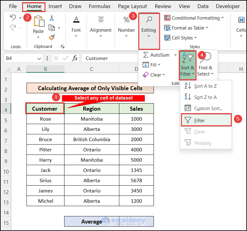
Steps:
- Filter the dataset to hide rows. To enable the Filter feature for the dataset, select any cell of the dataset.
- Go to the Home tab >> Editing menu >> Sort & Filter option >> Filter.
- Paste the formula in cell D15 to get the average of all cells in the range D5:D13.
=SUBTOTAL(1,D5:D13)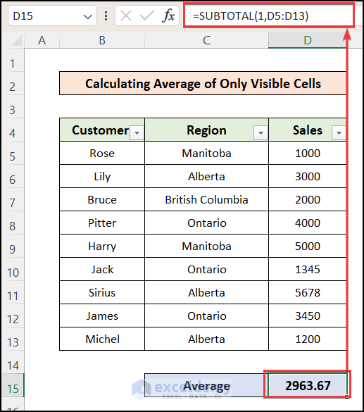
Formula Explanation
It returns a list or database. It offers 11 functions to perform by inserting the corresponding argument.
Syntax:
SUBTOTAL(function_num,ref1,[ref2],…)
- function_num = 1 to 11: Includes manually hidden rows but excludes filtered-out cells.
- function_num = 101 to 111: Excludes both manually hidden rows and filtered-out cells.
To exclude filtered-out cells only, we have used 1 in the function_num argument, and selected the full range of the dataset D5:D13 to calculate the average. Before filtering, we got the average of the full column.
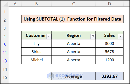
- Filter the data to check the output. If you want to get the average sales of any region, then click on the Filter icon on the Region column header.
- Mark any region where you want to calculate the average and unmark the rest.
- Press OK.

- See that the Average cell shows the average sales for only the Alberta region.
1.2 For Data with Hidden Rows
Steps:
- Insert the following formula into cell D15.
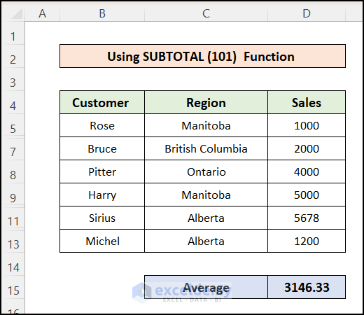
=SUBTOTAL(101,D5:D13)- Get the Average of the full column before hiding any rows.
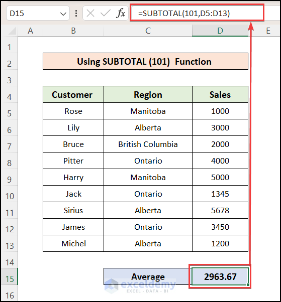
- Hide any row from the dataset. Suppose you have hidden the 6th, 10th, and 12th rows.
- See the Average cell, which gives the average value of the visible cells.
Method 2 – Using AGGREGATE Function in Excel
Steps:
- Hide some rows from the dataset.
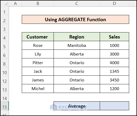
- Paste this formula into cell D15.
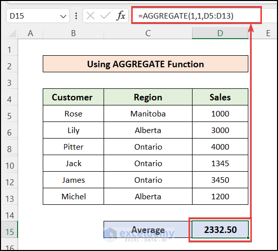
=AGGREGATE(1,1,D5:D13)Formula Breakdown:
Syntax:
AGGREGATE(function_num, options, array, [k])
- Insert function_num = 1 to calculate the average value of the selected data range.
- Insert options = 1 to exclude the hidden rows from the calculations.
- Select array = D5:D13 to calculate the average of this data range, excluding hidden rows.
- You got the average of only the visible cells in the selected data range.
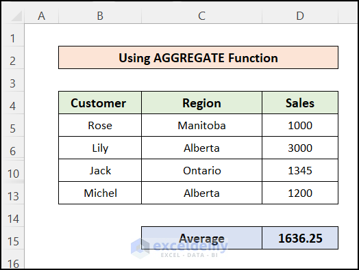
- Hide one or more rows of the dataset to check whether the formula works or not. We hidden the 8th and 12th rows, and the average value is changed which is the average of only the visible cells.
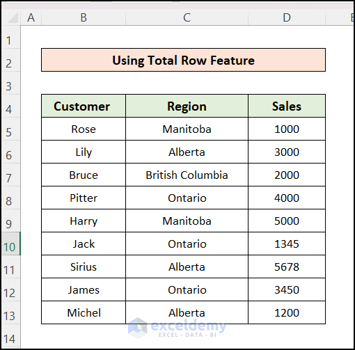
Method 3 – Average Visible Cells Using Total Row Feature of Excel Table
Steps:
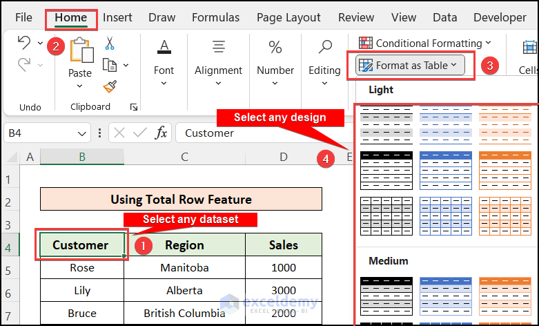
- You have to convert the dataset into an Excel table.
- To make a table, select any cell of the dataset.
- Go to the Home tab.
- Select the Format as Table option and there will be a list of table designs.
- Select any design from the options.
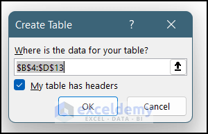
- After selecting a design for the table, a pop-up window named Create Table will appear.
- You will see here the range of table cells inserted already.
- Press OK.
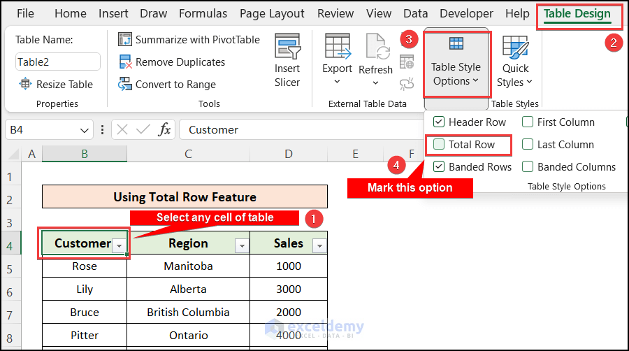
- The dataset will be converted into an Excel table.
- Select any cell of the table, and a new tab named Table Design will be created in the top ribbon.
- Go to the Table Style Options and mark the Total Row.
- There is a new row created at the bottom of the table showing the Total Sales. You can change it to show the average of the sales values.
- Click on cell D14 then a drop-down arrow will appear. Click on the arrow.
- Select the Average option.
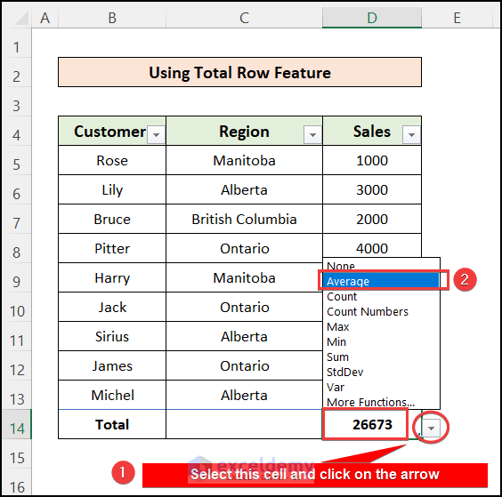
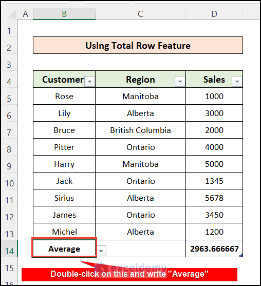
- Click on the cell B14 and rename it as Average.
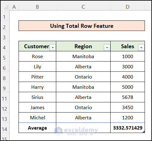
- Cell D14 shows the average value of the visible cells.
- Hide some rows to check whether the average cell value changes or not.
Things to Remember
- Use function_num 1 when you use the filtered dataset to exclude the filtered-out rows from the average calculation.
- Use function_num 101 when you want to exclude the manually hidden rows from the average calculation.
Download Practice Workbook
You can download the practice workbook from here:
Related Articles
- How to Find Average of Specific Cells in Excel
- How to Find Average with Blank Cells in Excel
- How to Exclude a Cell in Excel AVERAGE Formula
- How to Calculate Average of Multiple Ranges in Excel
- How to Average a Column in Excel
- How to Calculate Average of Multiple Columns in Excel
- How to Fix Divide by Zero Error for Average Calculation in Excel
- How to Ignore #N/A Error When Getting Average in Excel
- [Fixed!] AVERAGE Formula Not Working in Excel
<< Go Back to Conditional Average | Calculate Average | How to Calculate in Excel | Learn Excel
Get FREE Advanced Excel Exercises with Solutions!
