Method 1 – Using SUM and COUNTIF Functions to Calculate Average of Text in Excel
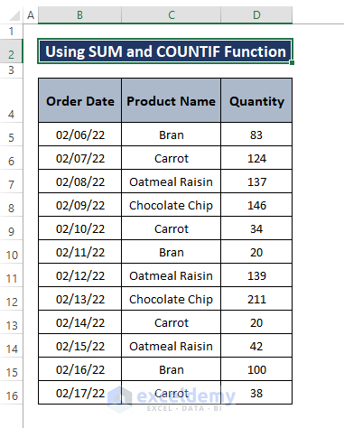
To calculate the average number of text, we have to first count the times a particular product appears in the entries. Then calculate its average using the simple average formula (i.e., count/total count). We will use the following dataset as our sample.
 Steps:
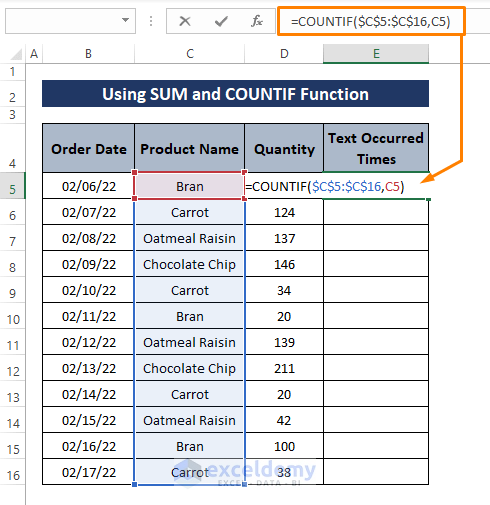
- To count the times of appearance, use the following formula in any adjacent blank cell (i.e., E5).
=COUNTIF($C$5:$C$16,C5)The COUNT function has a syntax of COUNTIF (range, criteria). The formula counts the criteria (i.e., E5) among all the Product Names (i.e., C5:C16) and returns the occurred times. In the formula, we use absolute references to lock the range for each cell.
- Press ENTER and drag the Fill Handle to display all the count numbers in the cells.
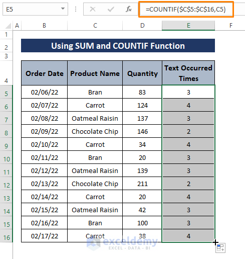
After applying the Fill Handle count numbers will appear in all cells. You can use the formula for counting any text appearances in a dataset.
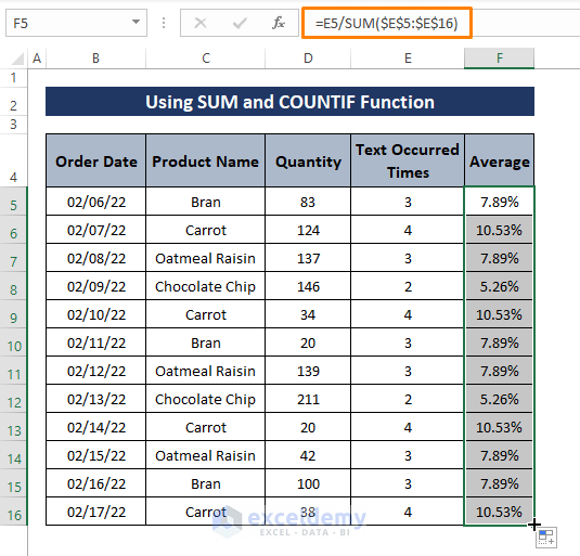
- We can now calculate the average of texts. Add the below formula in any adjacent cell.
=E5/SUM($E$5:$E$16)The formula divides the count numbers by the total count of products that appeared in the dataset.
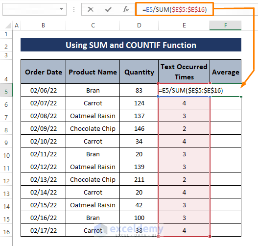
- Hit ENTER and drag the Fill Handle. The average values of Product Names appear in all cells as shown in the image below.
Read More: How to Average Filtered Data in Excel
Method 2 – Using a Combined Formula While Assigning Value to the Text
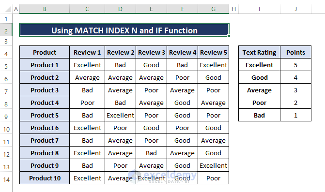
We have 10 Products along with their reviews. We pick those product reviews and want to calculate the average of text by assigning review texts a value.
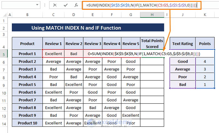
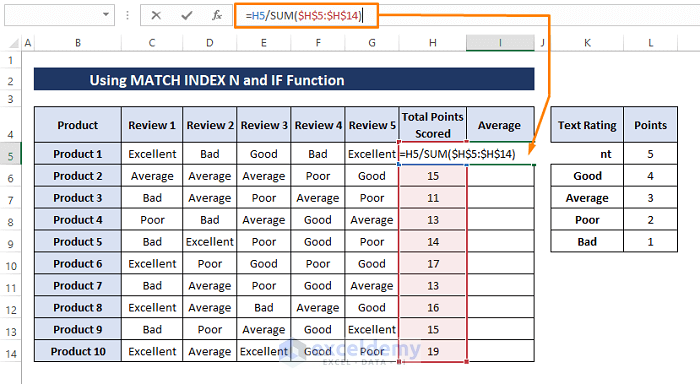
- Enter the following formula in any blank cell (i.e., H5).
=SUM(INDEX($L$5:$L$9,N(IF(1,MATCH(C5:G5,$J$5:$J$9,0)))))The formula consists of multiple functions such as SUM, MATCH, IF, N, and INDEX.
The IF function performs a logical_test (i.e., 1) and applies the MATCH function in case of TRUE outcomes. The MATCH function assigns values depending on the lookup_value matchings. For instance, it matches Excellent to point 5 and Bad to point 1.
The MATCH function takes the reviews (C5:G5) as lookup_value and matches them to an array ($J$5:$J$9) for an absolute match.
The N function converts a value into a number. In this formula, the resultant number passes to the INDEX function as the row_num. Then the SUM function combines all the array points in cell H5.
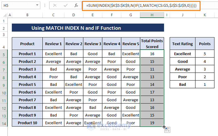
- The custom formula used in Step 1 is an array formula.
- Press CTRL+SHIFT+ENTER to display the sum. Drag the Fill Handle to show all the sum in other cells depicted in the following image.
- After getting the total sum points against reviews, apply the average formula in the adjacent cell (i.e., I5).
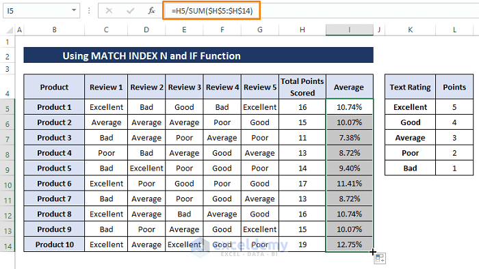
=H5/SUM($H$5:$H$14)This formula calculates the average of each product by dividing it by total points.
- Use ENTER to apply the formula in cells.
- Drag the Fill Handle to make all the averages visible similar to the image below.
 You can use any text and assign values or points in order to calculate their averages. Assigning values to texts gives a relative understanding of how a product is performing compared to others.
Download Excel Workbook
Related Articles
- How to Do Subtotal Average in Excel
- How to Calculate Sum & Average with Excel Formula
- How to Calculate Average and Standard Deviation in Excel
- How to Calculate Average Deviation in Excel Formula
- How to Calculate Average Excluding Outliers in Excel
- How to Average Negative and Positive Numbers in Excel
<< Go Back to Conditional Average | Calculate Average | How to Calculate in Excel | Learn Excel
Get FREE Advanced Excel Exercises with Solutions!

Hello! correct me if i’m wrong but doing the first method, even though formula wise it’s correct it will give wrong value has you are suming the range and adding the same value whenever the same name appears.
So counting the name Brian, you have it in the array only 3 times but if you sum the nnumber of time that name is showed it’s counting 9, so the percentage will be incorrect.
Hi TIAGO,
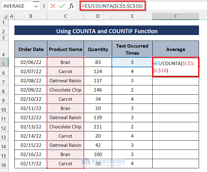
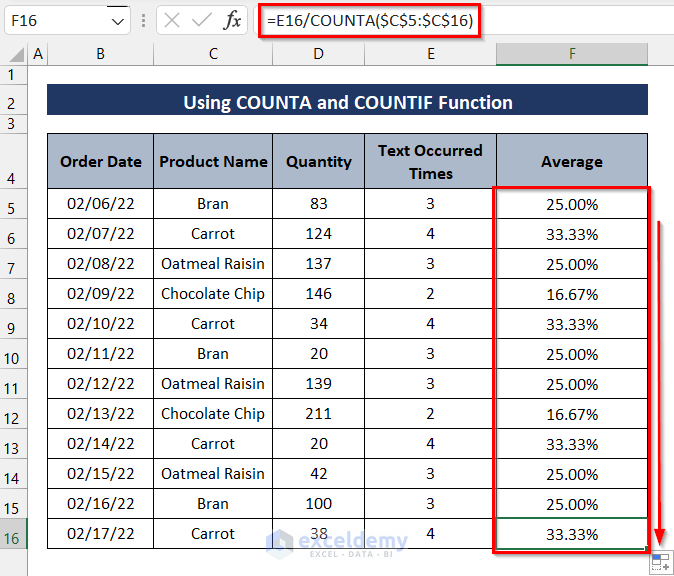
Thanks for your comment. I am replying to you on behalf of ExcelDemy. You can get the correct value by using the COUNTA function instead of the SUM function. Let’s see the steps.
Step-01: Write the following formula in the selected cell.
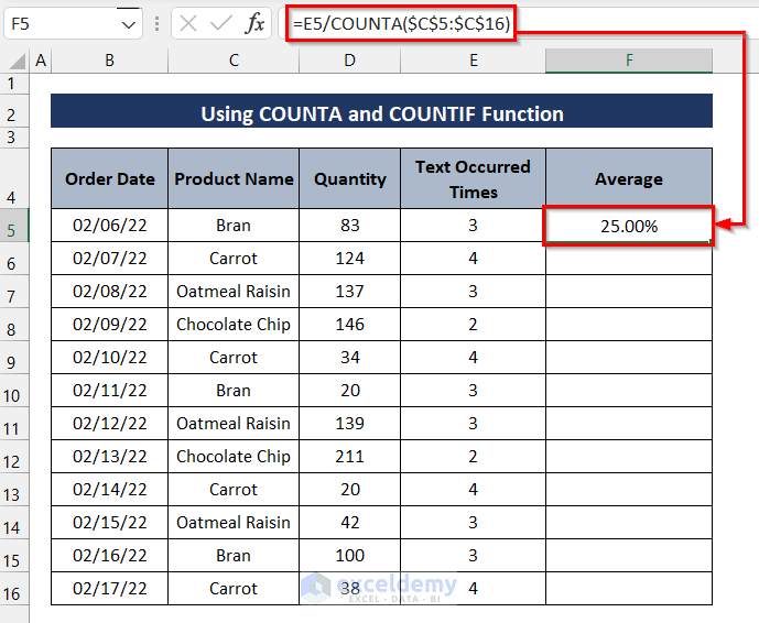
=E5/COUNTA($C$5:$C$16)Step-02: Press Enter to get the Average.
Step-03: Drag the Fill Handle down to copy the formula to the other cells.
I hope this will help you to solve your problem. Please let me know if you have other queries.
Regards
Mashhura,
ExcelDemy.