In this article, we will comprehensively cover calculating the average in Excel, particularly using the AVERAGE function to find the average of certain numbers, rows/columns and a range of cells.
We’ll also provide practical examples, such as finding the average of the top or bottom 5, the average based on single or multiple criteria, and use of the AVERAGEA, AVERAGEIF, and AVERAGEIFS functions.
Download Practice Workbook
How to Calculate the Average for Different Cases in Excel
Example 1 – Finding the Average of Certain Numbers
To calculate the average of certain numbers, provide the numbers as the arguments of the AVERAGE function. Add as many as you need.
- Enter the following formula in cell C5 (or modify it to fit your needs):
=AVERAGE(4,6,8,10,12)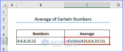
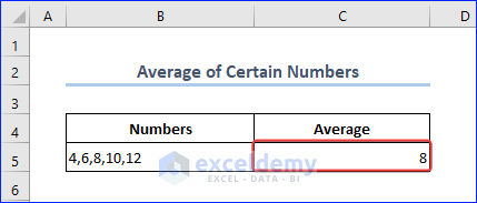
- Press ENTER to return the average.
Example 2 – Finding the Average of a Row or Column
To calculate the average of a whole column, use the following syntax in the formula:
=AVERAGE(C:C)- Enter the formula above in cell I9 and press ENTER to get the average of column C.
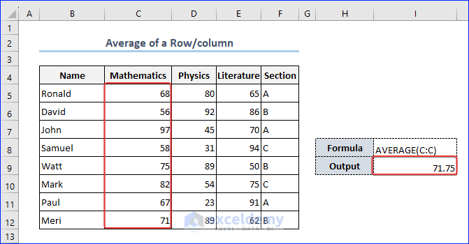
Note: Since we are calculating the average of Column C, we have given the argument C:C. Modify this according to your requirements.
To find the average of a row, modify the formula to something like AVERAGE(3:3). Change the argument 3:3 to the row for which you want to find the average.
Read More: How to Calculate Average of Multiple Ranges in Excel
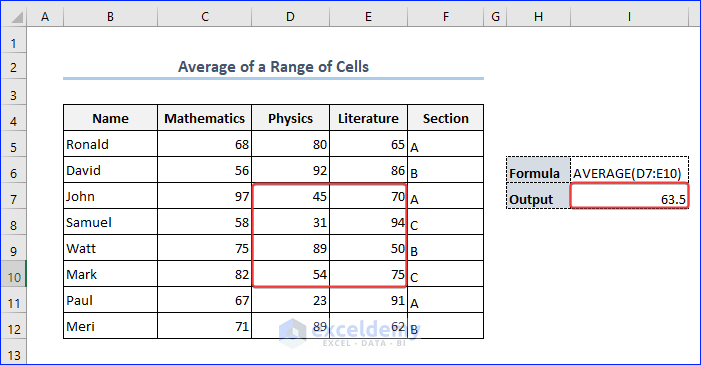
Example 3 – Finding the Average of a Range of Cells
To find the average of a range of cells, use the formula below:
Here, D7 is the starting point of the range, and E10 is the end of the range.
- Modify this formula according to your sheet then press ENTER to get the output.
In our dataset, the output is as in the following image.
Read More: How to Average a Column in Excel
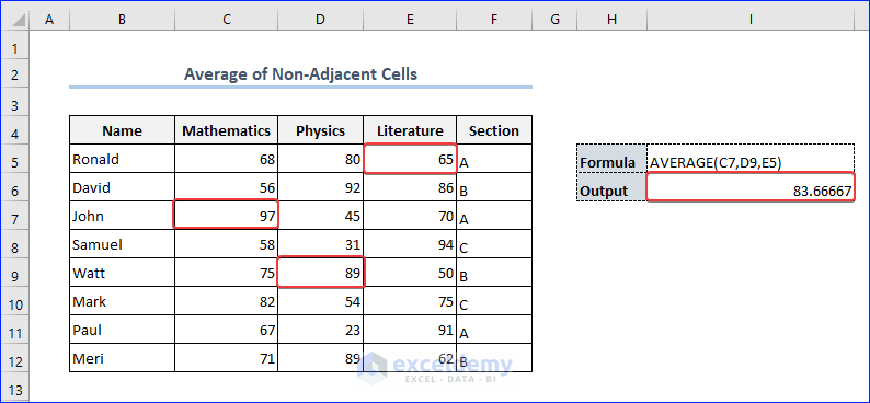
Example 4 – Finding the Average of Non-Adjacent Cells
To calculate the average of non-adjacent cells, provide the cell addresses as arguments in the AVERAGE function.
For example, to find the average of the numbers in cells C7, D9 and E5, enter the following formula in a cell and press ENTER:
The result is as follows:
Read More: How to Calculate Average of Multiple Columns in Excel
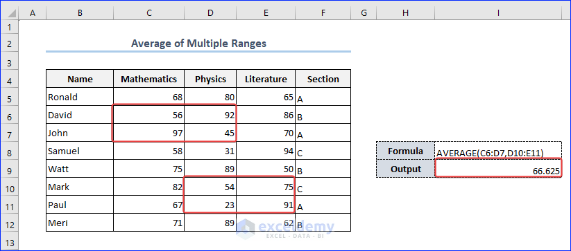
Example 5 – Finding the Average of Multiple Ranges
To find the average of the numbers in different ranges, provide them as the arguments in the AVERAGE function, like in the following formula:
=AVERAGE(C6:D7,D10:E11)- Modify the arguments (Ranges) in the above formula and enter it in a cell in your worksheet.
- Press ENTER to get the output.
Our output looks like the following image.
Read More: How to Find Average with Blank Cells in Excel
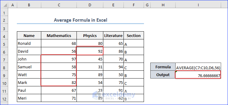
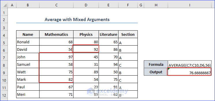
Example 6 – Using the AVERAGE Function with Mixed Arguments
We can use the AVERAGE function with mixed arguments (any combination of numbers, cell references, ranges or even functions), like in the following formula:
=AVERAGE(C7:C10,D6,56)- Modify the above formula according to your sheet and press ENTER to get the output.
Read More: How to Fix Divide by Zero Error for Average Calculation in Excel
Practical Examples of Calculating the Average in Excel
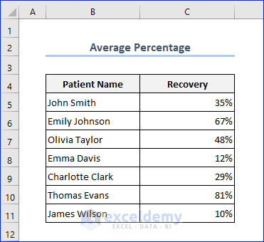
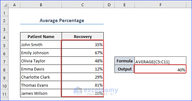
Method 1 – Finding the Average Percentage
Let’s find the average percentage in the dataset below.
- Enter the following formula into a cell and press ENTER:
=AVERAGE(C5:C11)The output is returned as a percentage.
Read More: [Fixed!] AVERAGE Formula Not Working in Excel
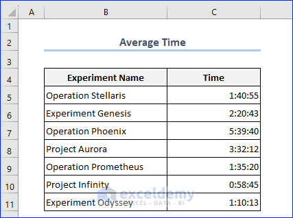
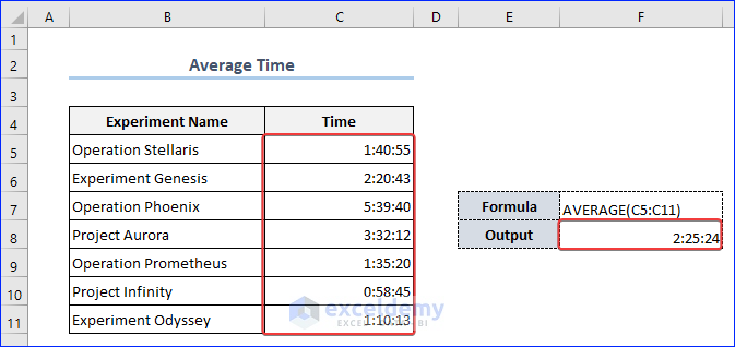
Method 2 – Finding the Average Time
Let’s calculate the average time in the dataset below.
- Enter the following formula in a blank cell and press ENTER.
=AVERAGE(C5:C11)The output is returned in the same time format as the argument.
Read More: How to Calculate Average and Standard Deviation in Excel
Method 3 – Finding the Average Without Zeros
To find the average without considering any zero values, we will use the AVERAGEIF function.
Let’s find the average Weight in the dataset below, ignoring the zero values.
- Enter the following formula in a blank cell:
=AVERAGEIF(E5:E10,"<>0")- Press ENTER to return the result.
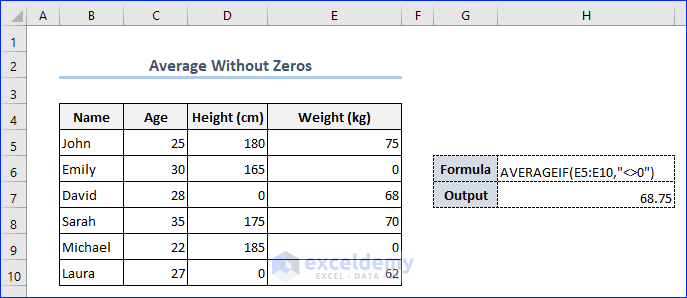
Note: While finding the average of cells, keep in mind the difference between empty cells and those containing the value zero, especially if you have cleared the option “Show a zero in cells that have zero value” in the Excel desktop application.
Method 4 – Finding the Average of the Best 5 / Worst 5
4.1 – Finding the Average of the Best 5
- We will combine the AVERAGE and LARGE functions to find the average of the best 5 values in a range.
=AVERAGE(LARGE(C5:C12, {1,2,3,4,5}))- Use the formula in a cell and press ENTER.
The output will be similar to the image below.
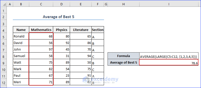
Formula Breakdown
- LARGE(C5:C12, {1,2,3,4,5}) : The LARGE function finds the top 5 values in the array C5:C12.
- AVERAGE(LARGE(C5:C12, {1,2,3,4,5})) : Finds the average of the array returned by the LARGE function.
Read More: How to Add Average Line to Excel Chart
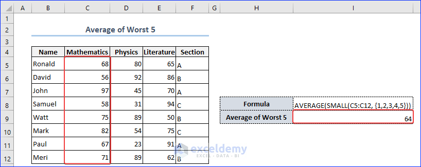
4.2 – Finding the Average of the Worst 5
To find the average of the smallest 5 values, we will combine the AVERAGE and SMALL functions.
=AVERAGE(SMALL(C5:C12, {1,2,3,4,5}))- Use the formula above in a cell and press ENTER to get the output.
The output will look similar to the following image:
Method 5 – Finding the Average Including Text Values Using the AVERAGEA Function
If our dataset contains both numbers and text, we can use the AVERAGEA function to calculate the average.
- Use the following formula in your worksheet to get the average of the dataset, even though it contains text:
=AVERAGEA(B5:C12)- Use the formula above to return the average of the numbers in the range.
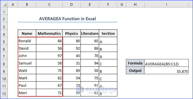
Note: The AVERAGEA function considers text values as 0 when calculating the average. The result will therefore not be the same as from calculating just the numbers.
Read More: How to Use VBA Average Function in Excel
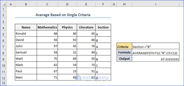
Method 6 – Finding the Average Based on a Single Criterion Using the AVERAGEIF Function
To find the average based on a single criterion, use the formula below in cell I9:
=AVERAGEIF(F5:F12,"B",C5:C12)Here, the function takes the first and second arguments as the criteria to calculate the average, while the third argument is the range where the function will apply the criteria.
After pressing ENTER, the result below is returned.
Read More: How to Find Average with OFFSET Function in Excel
Method 7 – Finding the Average Based on Multiple Criteria Using the AVERAGEIFS Function
To find the average based on multiple criteria, use the formula below:
=AVERAGEIFS(E5:E12,F5:F12,"A",E5:E12,">=70")Here, the AVERAGEIFS function has 3 arguments: the first is the range where the function will calculate the average, and the second and third are the criteria based on which the function will calculate the average.
- Press ENTER to return the result.
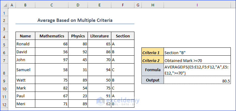
Note: We have given 2 criteria in the AVERAGEIFS function. Use as many as you need in your formulas.
Read More: How to VLOOKUP and AVERAGE Specific Values in Excel
[Fixed!] AVERAGE Formula Not Working in Excel
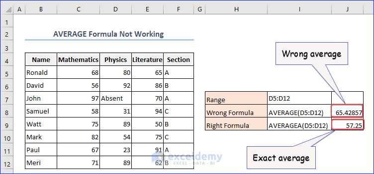
If the dataset that you are using to calculate the average using the AVERAGE function contains non-numeric data, then you won’t get the exact average of the data.
In the image below, the data includes a non-numeric value (Absent) in Column D. If you calculate the average using the AVERAGE function, you will get a value which is not the actual average of the data. So we’ll use the AVERAGEA function to calculate the average in this case instead.
Enter the following formula containing the AVERAGE function in a blank cell to get the wrong average:
=AVERAGE(D5:D12)The correct formula to calculate the exact average is as follows:
=AVERAGEA(D5:D12)The difference between the output of these 2 formulas is as follows:
AVERAGE vs AVERAGEA vs AVERAGEIF vs AVERAGEIFS
- The AVERAGE function in Excel calculates the arithmetic mean of a range of cells.
- The AVERAGEA function is similar to AVERAGE, but it includes all values in the specified range, treating text and logical values as zeros.
- The AVERAGEIF function calculates the average of a range of cells that meet a specified condition.
- The AVERAGEIFS function is an extension of AVERAGEIF and allows you to calculate the average based on multiple criteria.
Things to Remember
- If the arguments of the AVERAGE function refer to cells that contain #VALUE! errors, the formula will also result in a #VALUE! error.
- If the range of cells you are trying to calculate has no numeric values, the AVERAGE formula will return a #DIV/0! error.
- The AVERAGEIFS function requires at least 2 criteria to work properly.
- The AVERAGE function can take exact values, cell references, and ranges as arguments.
Frequently Asked Questions
1. What is the difference between the AVERAGE and AVERAGEA formulas in Excel?
The AVERAGE formula calculates the average of only numeric values, while the AVERAGEA formula includes all values in the range, treating non-numeric values as zero for the purpose of averaging.
2. Is it possible to include only certain cells from a range in the average calculation?
Yes, use the AVERAGEIF or AVERAGEIFS function to find an average with conditions.
3. Does the AVERAGE formula include or exclude zero values?
The AVERAGE formula includes zero values in the calculation. When you use the AVERAGE formula, it considers all numeric values within the specified range.
Average Formula in Excel: Knowledge Hub
<< Go Back to How to Calculate in Excel | Learn Excel
Get FREE Advanced Excel Exercises with Solutions!
