How to Find Average with OFFSET Function in Excel (3 Examples)

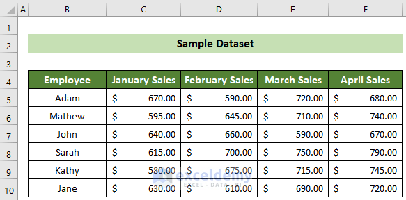
Suppose we have the dataset below of 6 employees’ sales in the first 4 months of a year. Let’s calculate the average sales for individual months and also the average sales of individual employees for the full 4 months using the OFFSET and AVERAGE functions.

Method 1 – Calculate Average of Any Number of Rows/Columns Using the OFFSET Function

Steps:

• Click on cell G5 and insert the following formula:

• Press Enter.

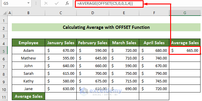
The average sales for the employee Adam is returned.

• Place your cursor in the bottom right position of the cell.
• Drag the Fill Handle down to copy the formula to the rest of the cells in the series.

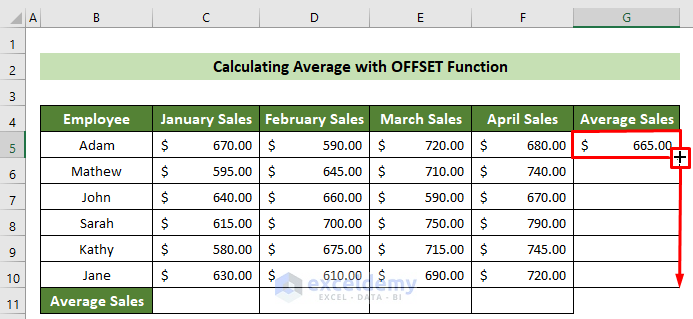
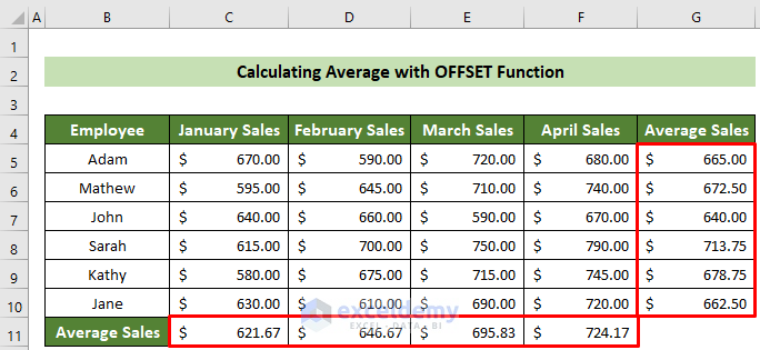
The average sales for all employees are returned.

• To calculate the monthly average sales, click on cell C11 and insert the formula below:

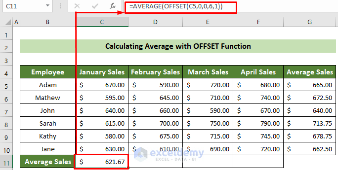
• Press Enter.
• Drag the Fill Handle right to copy the same formula for all the other months.

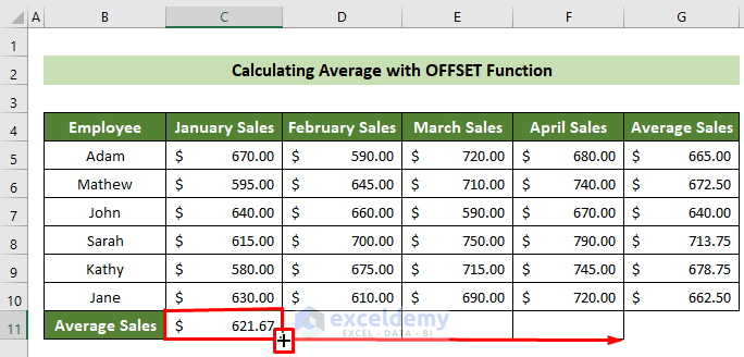
The result will look like this:

Read More: How to Calculate VLOOKUP AVERAGE in Excel

Method 2 – Combining COUNT and OFFSET Functionsto Calculate Average of Last N Number of Rows/ Columns

Using the OFFSET function in combination with the COUNT function, we can calculate the average for N number of rows or columns dynamically.

2.1 – Average of Last N Rows

Steps:

• Set the N value as 2 in cell C13.
• Click on cell B13 and enter the following formula in the formula bar:

• Press Enter.

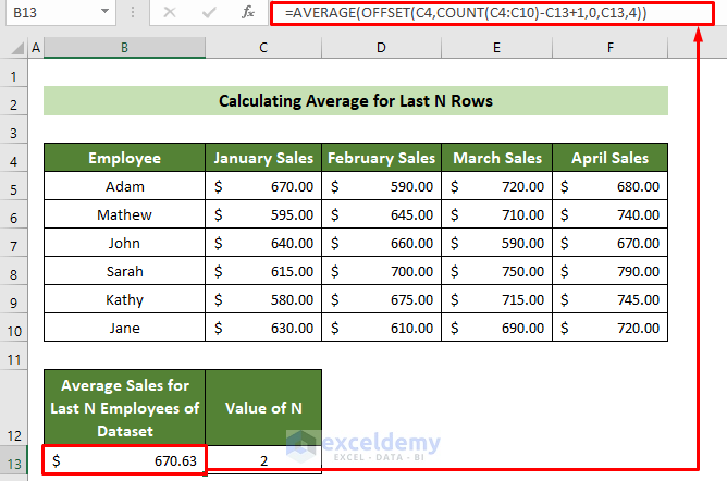
The average sales of the last two employees for all 4 months is returned. Change the value of N as required and the AVERAGE function will automatically return the exact result.

2.2 – Average of Last N Columns

Let’s calculate the average for all employees but only for the last two months.

Steps:

• Set the N value as 2 in cell C13.
• Insert the following formula in cell B13 and press Enter:

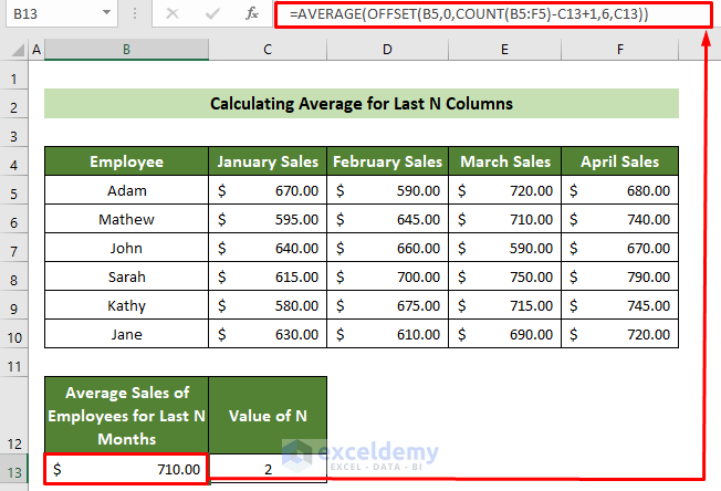
The average sales for all employees for the last two months is returned. To calculate the average for any other number of months, simply change the N value accordingly.

Method 3 – Using OFFSET and ROW Functions to Calculate Average for Every N Number of Rows/Columns

You might need to calculate average sales in a consecutive manner, i.e. for every N number of rows or columns.

3.1 – Average of Every N Number of Rows

Let’s calculate average sales for every two employees in the dataset using the ROW function together with the OFFSET function.

Steps:

• Click on cell C13 and insert the following formula:

• Press Enter.

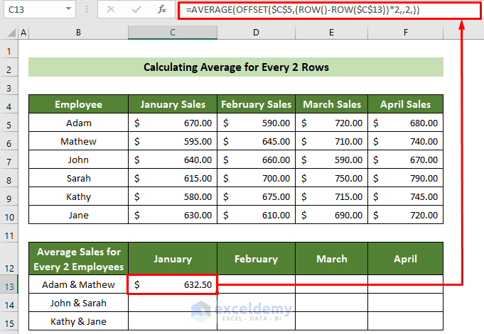
The January average sales for Adam and Mathew is returned.

• Drag the Fill Handle down to copy the formula to the cells below.

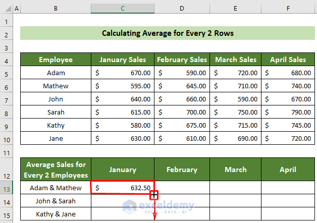
For the other months, dragging the Fill Handle won’t work properly due to our use of absolute references.

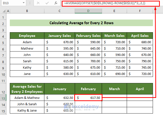
• So, for the February sales average for every two employees, click on cell D13 and insert the following formula:

• Press Enter.

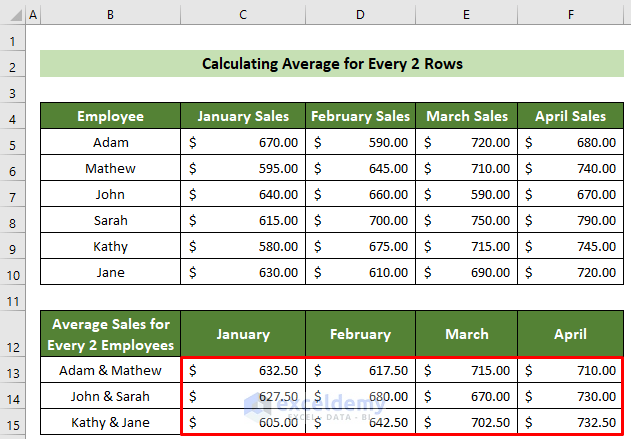
• Repeat the same procedure for all the other cells, modifying your formula in the same way for every month.

The averages for every two rows every month are returned.

Read More: How to Average Every Nth Row in Excel

3.2 – Average of Every N Number of Columns

We can calculate the average for every employee every two months by combining the COLUMNS function with the OFFSET function.

Steps:

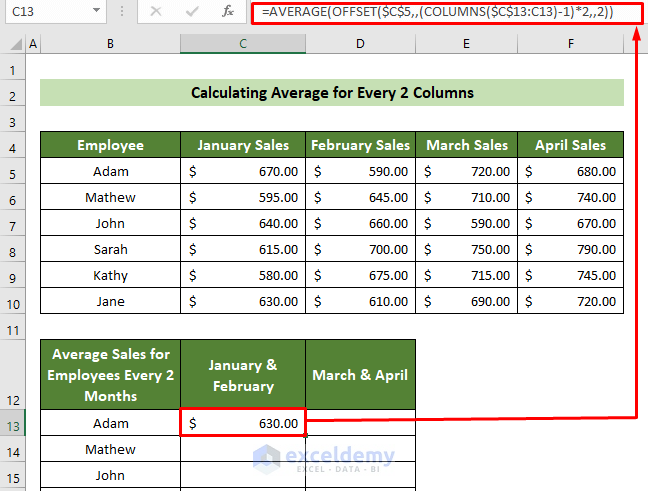
• Click on cell C13 and insert the following formula:

• Press Enter.

• Drag the Fill Handle right to repeat the same result for the next two months.

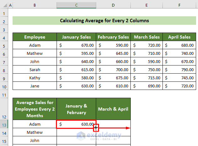
Being an absolute reference, the formula won’t work properly if you drag the Fill Handle below for other employees.

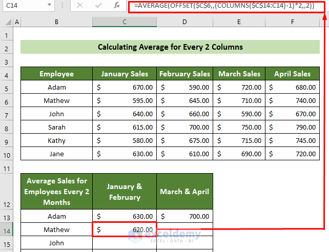
• For the next employee, click on cell C14 and enter the formula below in the formula bar:

• Press Enter.

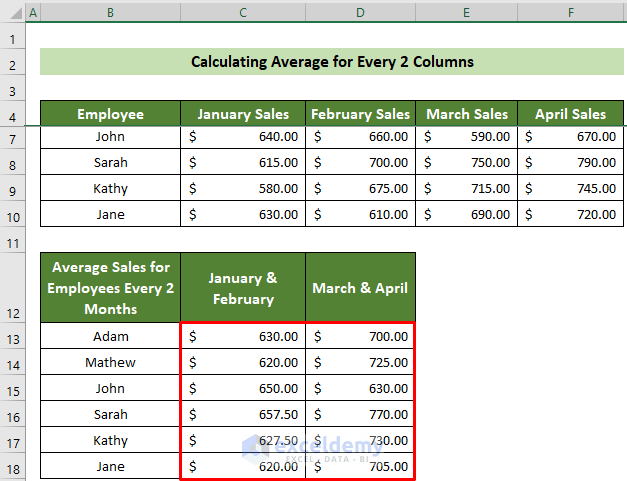
• Repeat the same dragging approach, changing the formula accordingly for each employee.

All employees’ average sales every two months are returned.

Things to Remember

• The OFFSET function will return a #VALUE! error if any argument is invalid, like a missing cell reference.
• The OFFSET function will return a #REF! error if you refer to any cell that is outside of the spreadsheet.

Download Practice Workbook

Related Articles