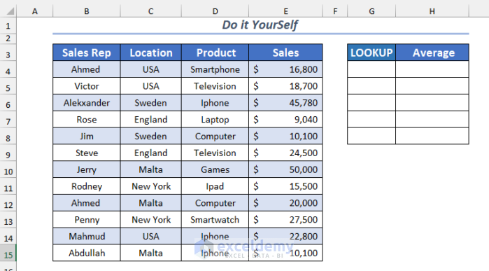
How to VLOOKUP and AVERAGE Specific Values in Excel

The sample dataset contains sales information on different regions.

Method 1 – Merge the VLOOKUP and AVERAGE Functions in Excel

Select a cell. We chose G4.
Enter the following formula in the selected cell or in the Formula Bar.

=VLOOKUP(AVERAGE(B4:B15),B4:C15,2,TRUE)

This function will look up the average sales value in the Sales column and will return the Sales Person’s name.

Press ENTER.
The salesperson’s name whose sales amount match the average sales will be displayed.

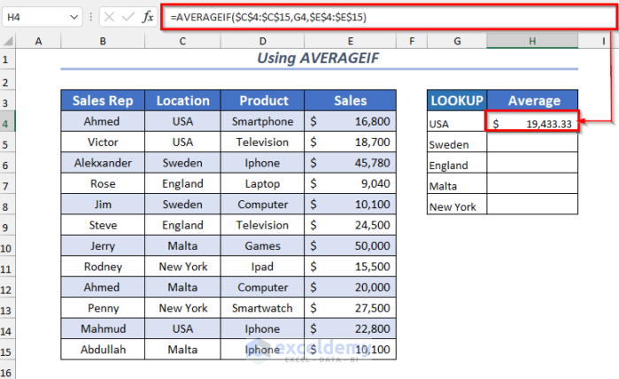
Method 2 – Using the AVERAGEIF Function to VLOOKUP the AVERAGE of Specific Criteria.

Select a cell. We used H4.
Enter the following formula in the selected cell or in the Formula Bar.

=AVERAGEIF($C$4:$C$15,G4,$E$4:$E$15)

C4:C15 is the Location column; G4 is the criterion; E4:E15 in the Sales column is the average_array.

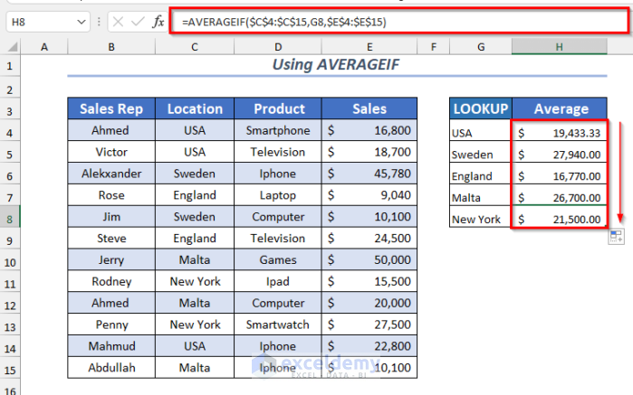
Press ENTER.

This is the output.

Use the Fill Handle to AutoFill the rest of the cells.

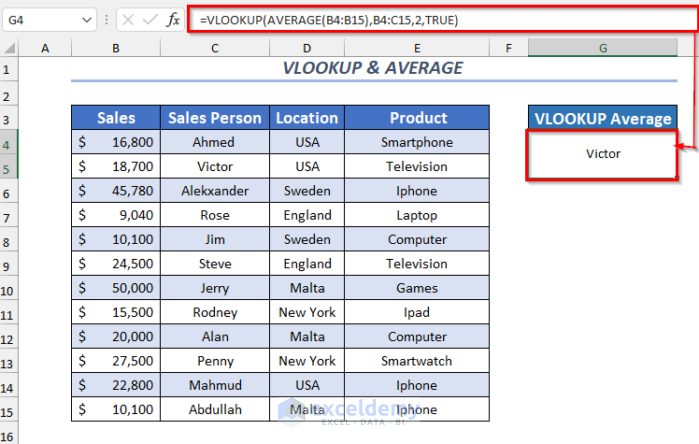
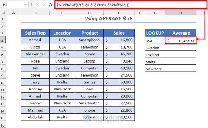
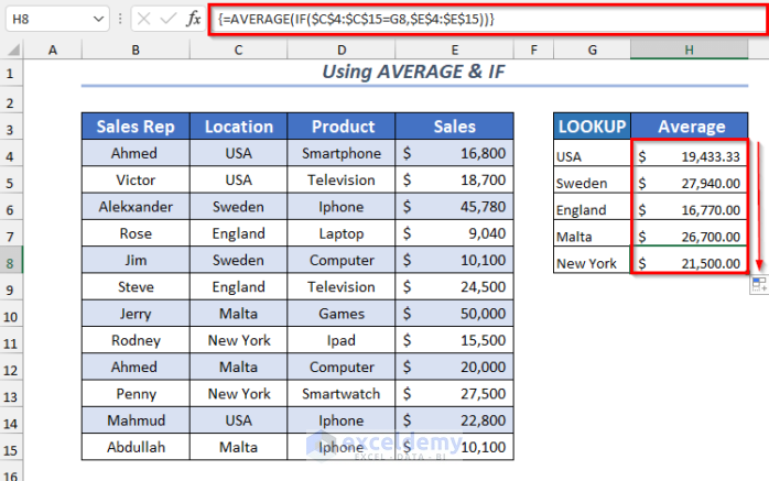
Method 3 – Combining the AVERAGE and IF Functions

Select a cell. Here, H4.
Enter the following formula in the selected cell or in the Formula Bar.

=AVERAGE(IF($C$4:$C$15=G4,$E$4:$E$15))

The IF function will get the values for G4 cell using a logical_test. The AVERAGE function will calculate the average values in USA.

Press ENTER.

This is the output.

Use the Fill Handle to AutoFill the rest of the cells.

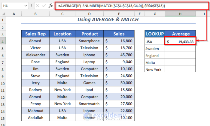
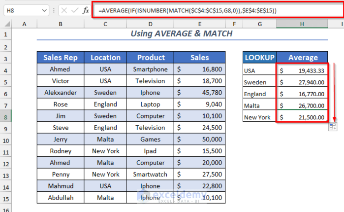
Method 4 – Joining the AVERAGE and MATCH Functions to Lookup Values and Calculate the Average

Select a cell. We used H4.
Enter the following formula in the selected cell or in the Formula Bar.

=AVERAGE(IF(ISNUMBER(MATCH($C$4:$C$15,G4,0)),$E$4:$E$15))

The MATCH function will match the values for G4 from the Location column and pass the value to ISNUMBER. The IF function will apply the logical_test in the range E4:E15.

Press ENTER.

This is the output.

Use the Fill Handle to AutoFill the rest of the cells.

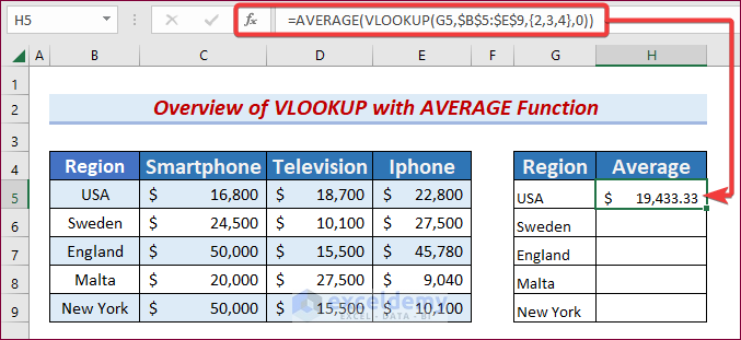
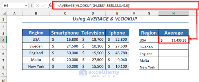
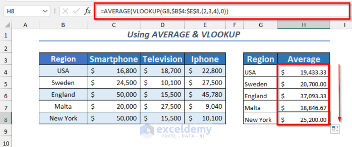
Method 5 – Using AVERAGE and VLOOKUP

Select a cell. We chose H4.
Enter the following formula in the selected cell or in the Formula Bar.

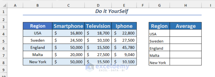
=AVERAGE(VLOOKUP(G4,$B$4:$E$8,{2,3,4},0))

The VLOOKUP function will get the values for G4 from the Location column for the selected range B4:E8. The AVERAGE function will calculate the average values.

Press ENTER.

This is the output.

Use the Fill Handle to AutoFill the rest of the cells.

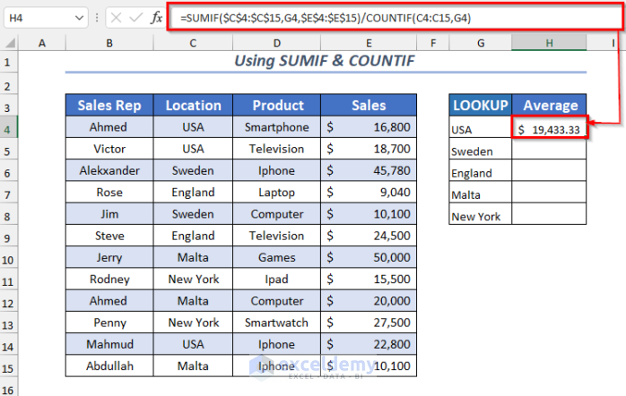
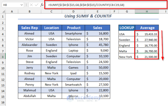
Method 6 – Merging the SUMIF and COUNTIF Functions

Select a cell. We used H4.
Enter the following formula in the selected cell or in the Formula Bar.

=SUMIF($C$4:$C$15,G4,$E$4:$E$15)/COUNTIF(C4:C15,G4)

The SUMIF function will get the values for G4 and calculate the sum of those values. The COUNTIF function will count the occurrences of G4 . The sum of the values will be divided by the count.