1. Combining Functions to Average Every Nth Row
Steps:
- Calculate the average of the data in the Sales column for every three rows.
- Write the following formula in cell D5.
=AVERAGE(OFFSET($C$5,(ROW()-ROW($D$5))*3,,3,))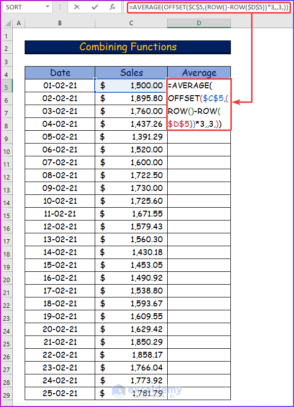
Formula Breakdown
- OFFSET($C$5,(ROW()-ROW($D$5))*3,,3,): The OFFSET function with the help of the ROW function will fetch the data starting from cell C5 for calculation. The row height is 3 so this function will collect three rows of height downward starting from cell C5.
- AVERAGE(OFFSET($C$5,(ROW()-ROW($D$5))*5,,5,)): Finally, the AVERAGE function will calculate the average of the values found from the previous steps.
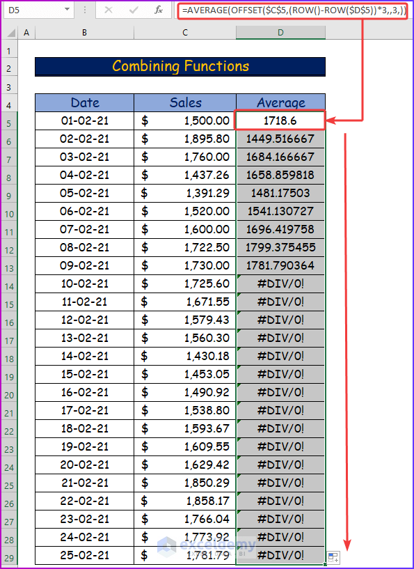
- Press Enter to see the average of the first three rows in cell D5.
- Use AutoFill to drag the formula to the lower cells of this column.
- See a numerical value, till the formula finds values for calculations.
- It will show #DIV/0! as an error.
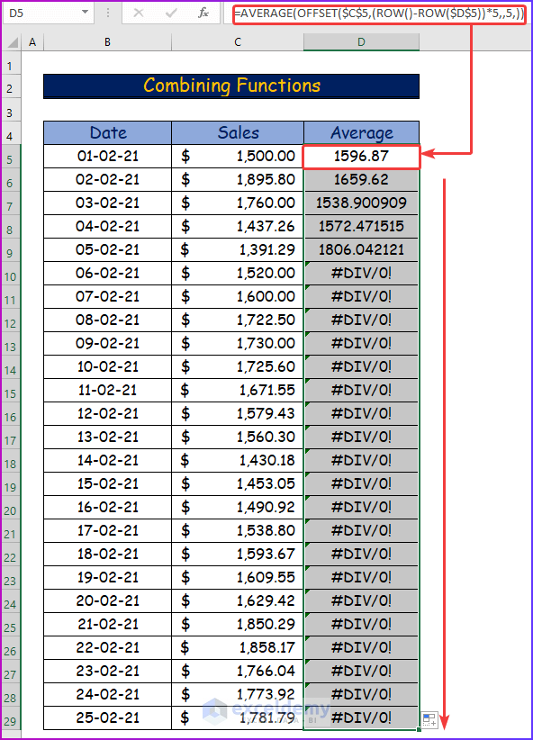
- Modify the formula a little bit, and you will see the average for every five rows.
Method 2 – Merging Functions to Average Every Nth Row
Steps:
- Determine the average sales for every three rows.
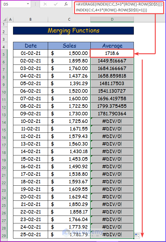
- In cell D5, use the following merging formula.
=AVERAGE(INDEX(C:C,5+3*(ROW()-ROW($D$5))):INDEX(C:C,4+3*(ROW()-ROW($D$5)+1)))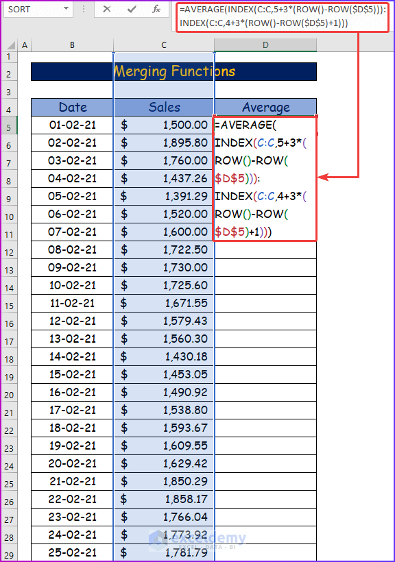
Formula Breakdown
- INDEX(C:C,5+3*(ROW()-ROW($D$5))): The INDEX function will find the value from the cell range or column C that falls in row 5. The row number is calculated using the ROW function.
- INDEX(C:C,4+3*(ROW()-ROW($D$5)+1)): The INDEX function will find the value from the third row of the data set, which is row 9 in the worksheet.
- AVERAGE(INDEX(C:C,5+3*(ROW()-ROW($D$5))):INDEX(C:C,4+3*(ROW()-ROW($D$5)+1))): The AVERAGE function will calculate the average of these two-row ranges found in the previous two sections.
- Press Enter to find out the average of the first three rows.
- Drag the same formula to the lower cells of the column by using the Fill Handle.
- The formula will show numerical values based on the size of your data set.
- After a certain period, it will show #DIV/0! as an error.
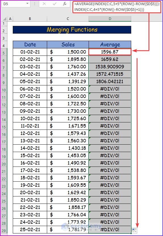
- Get the average for every five rows with the same formula; you have to modify the formula slightly.
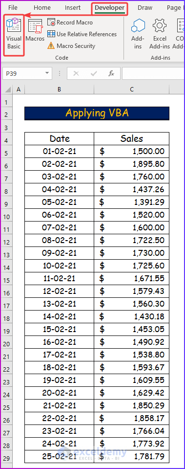
Method 3 – Applying VBA to Average Nth Row in Excel
Steps:
- Go to the Developer tab of the ribbon.
- From the Code group, select Visual Basic.
- The Visual Basic window will appear after the previous step.
- From the Insert tab choose Module.
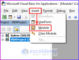
- Copy the following code into the module.
- We entered C5:C7 as the range to calculate the average that represents the first three rows of the data set.
Sub Average_Row_Range()
Dim x As Integer
'Assign the row range for calculating average
x = WorksheetFunction.Average(Range("C5:C9"))
'Displaying the result in a msgbox
MsgBox "The average of this row range is " & x
End Sub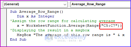
VBA Breakdown
- Naming the sub-procedure.
Sub Average_Row_Range()- Declare the variables.
Dim x As Integer- Assign the desired drow range for calculating the average.
x = WorksheetFunction.Average(Range("C5:C9"))- Use a message box to display the result.
MsgBox "The average of this row range is " & x- Save the code, and after keeping the cursor in the module press F5 or the Run button to run the code.
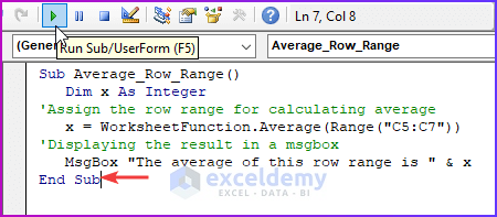
- You will see the average of the row range as a result after running the code.
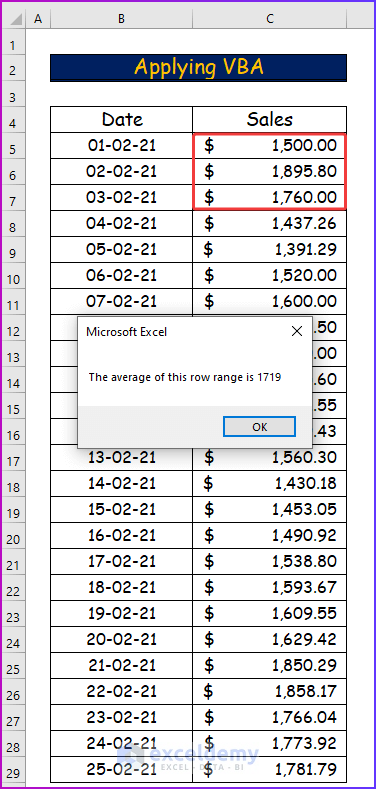
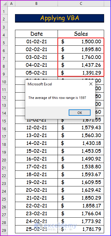
- Change the cell range in the code, and you will see the average for the first five rows in the message box.
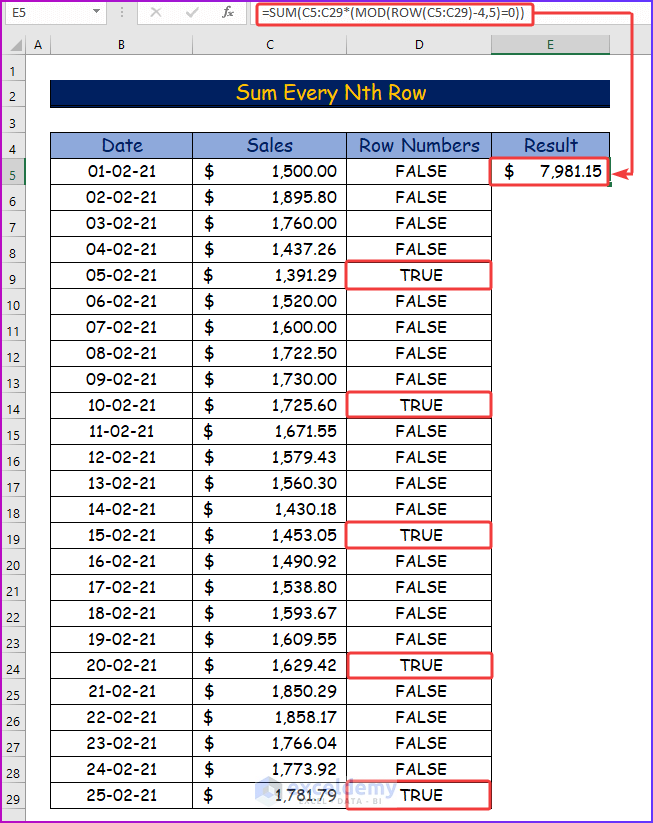
Sum Every Nth Row in Excel
Steps:
- Show the row numbers that will be summed up by those Excel functions.
- Insert the following formula into cell D5.
=MOD(ROW(C5)-4,5)=0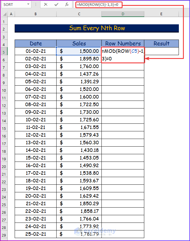
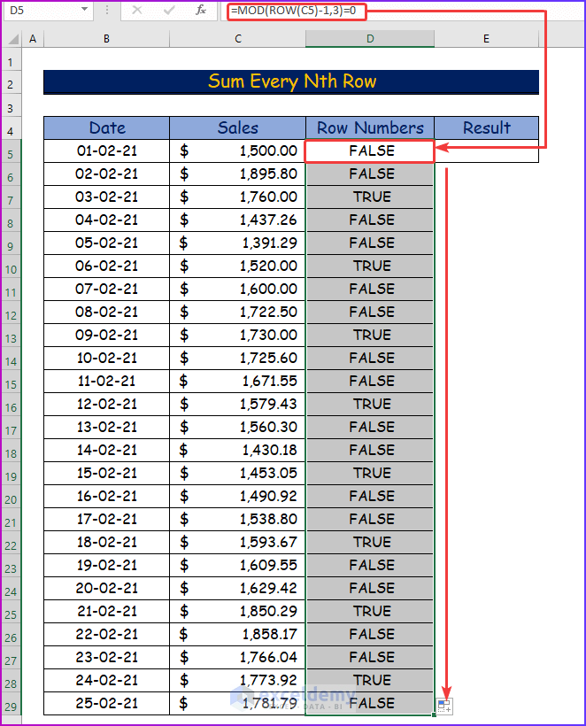
- Sum every third row from the data set, by using the above formula. You can see which row will be added to the main formula.
- Enter the following formula in cell E5, to sum up every third row and show the result.
=SUM(C5:C29*(MOD(ROW(C5:C29)-1,3)=0))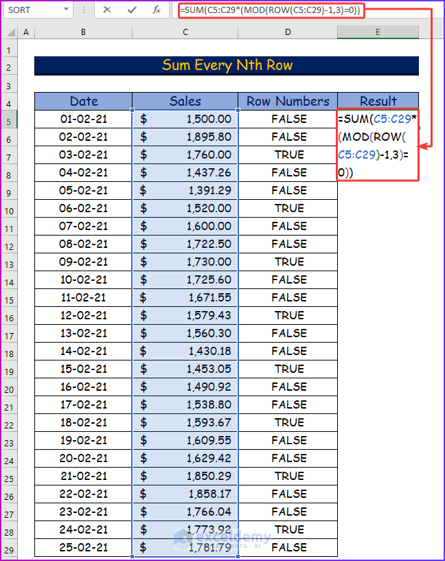
Formula Breakdown
- MOD(ROW(C5:C29)-1,3)=0: The MOD function will return 0 for every third row in the range C5:C29. As the data set does not start from cell A1, to find out the correct value of the row for this cell range, -1 has been used in the formula.
- SUM(C5:C29*(MOD(ROW(C5:C29)-1,3)=0)): The SUM function will sum up values from the rows that are true for the MOD function.
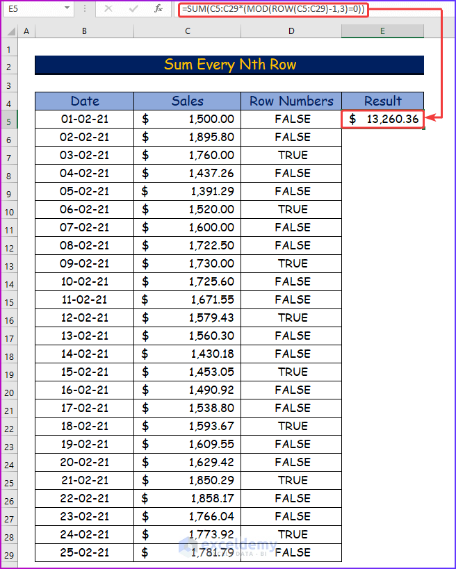
- Press Enter and see the desired result in cell E5.
- By modifying the above formula, you can determine the sum of every five rows from the data set.
Download Practice Workbook
You can download the free Excel workbook here and practice on your own.
Related Articles
- How to Calculate Average of Multiple Columns in Excel
- How to Calculate Average of Multiple Ranges in Excel
- How to Find Average with Blank Cells in Excel
- How to Average Only Visible Cells in Excel
- How to Find Average of Specific Cells in Excel
- How to Exclude a Cell in Excel AVERAGE Formula
- How to Fix Divide by Zero Error for Average Calculation in Excel
- How to Ignore #N/A Error When Getting Average in Excel
- [Fixed!] AVERAGE Formula Not Working in Excel
<< Go Back to Conditional Average | Calculate Average | How to Calculate in Excel | Learn Excel

