How to Calculate Average of Averages in Excel (with Easy Steps)

In Excel, we use to solve different types of real-life problems. One of them is to Calculate Average of Averages. In real life, an Average of averages or weighted average is needed in preparing results of a school or in paying wages to laborers concerning working hours, etc. However, you can prepare the reports containing weighted averages with a generic formula of excel. It is a straightforward process. In this article, I will describe how to Calculate Average of Averages in Excel with the necessary steps and illustrations.

Download Practice Workbook

Please download the practice workbook and practice yourself.

4 Suitable Steps to Calculate Average of Averages in Excel

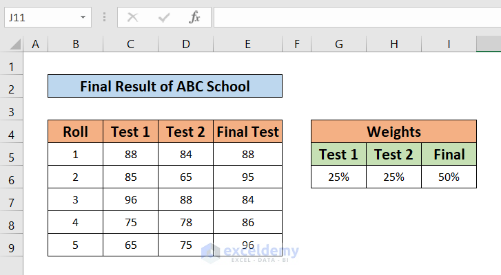
Before jumping into the steps, let’s introduce our dataset first. Here, we consider a dataset of the Final Result of ABC School. The dataset has 4 columns B, C, D, & E indicating Roll, Results of  Test 1, Test 2 & the Final Test. The dataset ranges from B4 to E9. Besides this table, we can see another table containing marks weightage in Test 1, Test 2, & Final Test respectively. Now, I will discuss how to Calculate Average of Averages in Excel with easy steps and illustrations. Follow the steps and increase your Excel skills.

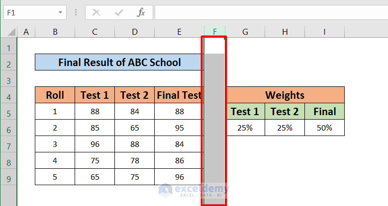
Step 1: Insert a New Column

• First, Select the F.
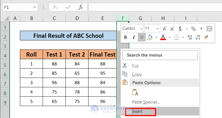
• Then Right-Click on the column.

• After that, Click the Insert.

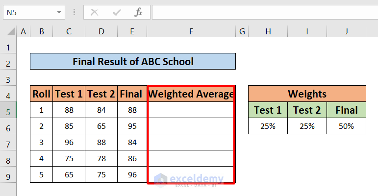
• You will find a new column is added. Name it “Weighted Average”.

Read More: How to Calculate Average in Excel (Including All Criteria)

Step 2: Apply SUMPRODUCT Formula to Calculate Weighted Average

• Now, Write down the following formula in the F5.

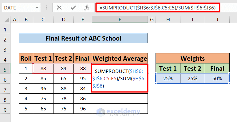
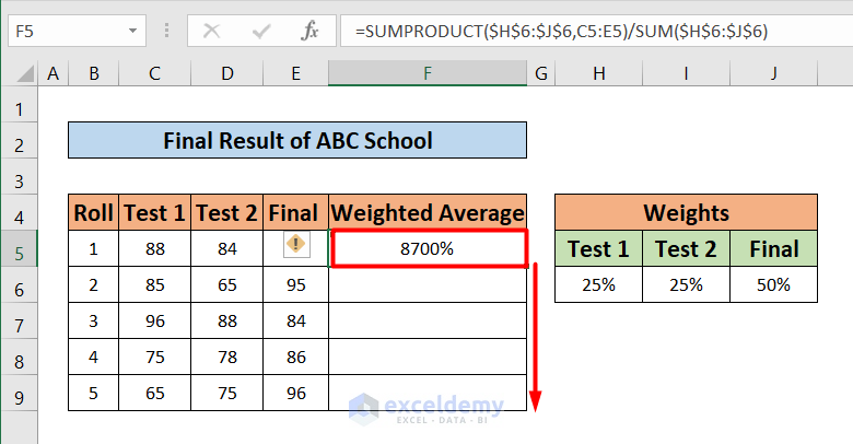
• You will find the result just like the picture given below.
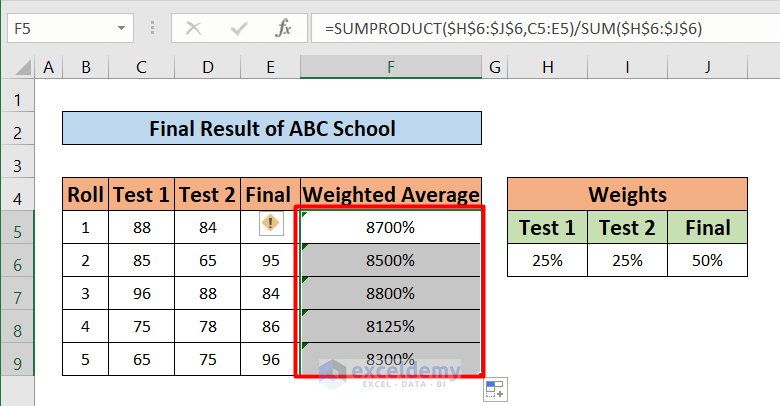
• Fill-handle the formula from F5 to F9.

• As a result, you will find the Weighted Average for every student.

Read More: How to Calculate Average of Multiple Ranges in Excel (3 Methods)

Similar Readings

• Calculate Average Percentage Increase in Excel
• How to Exclude a Cell in Excel AVERAGE Formula (4 Methods)
• [Fixed!] AVERAGE Formula Not Working in Excel (6 Solutions)
• Calculate the Average of an Array with VBA (Macro, UDF, and UserForm)
• How to Calculate Class Average in Excel (6 Easiest Methods)

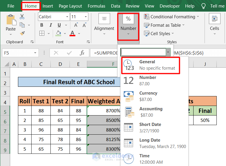
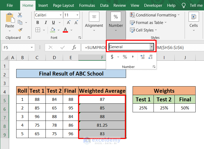
Step 3: Change Number Format to General

• Go to the Home tab in your Toolbar.
• Then, Select the Number
• After that, you will find the number format is in ‘Percentage’.

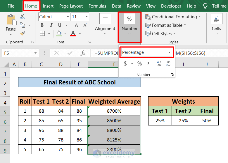
• Then, Change the number format to General.

• Hence, You will find the result just like the picture shown below.

Read More: How to Calculate Average Percentage of Marks in Excel (Top 4 Methods)

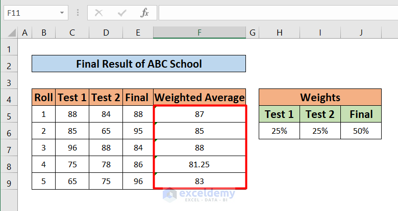
Step 4: Final Result of Average

• At last, you will find the result just like the picture given below.

Read More: How to Calculate Average, Minimum And Maximum in Excel (4 Easy Ways)

Things to Remember

• Use the absolute marks in the formula. Otherwise, an error will occur showing ‘#Div/0’.

Conclusion

In this article, I have tried to show how to Calculate Average of Averages in Excel. In addition, I have shown 4 handy steps to Calculate the Average of Averages. This method is very useful for both professionals and students or learners. I hope you have understood all the steps. If you have any queries, let me know in the comment sections.

Related Articles

• How to Calculate Daily Average from Hourly Data in Excel
• Average Every Nth Row in Excel (3 Ways)
• How to Calculate Average Growth Rate in Excel (3 Easy Methods)
• Average a Column in Excel (7 Easy Methods)
• How to Calculate Average Only for Cells with Values in Excel
• Calculate Average Rating in Excel (7 Methods)
• How to Calculate Average of Multiple Columns in Excel (6 Methods)