We need to calculate the average price in various business sectors or normal life frequently. Excel has made it easy to calculate the average price. There are various formulas in Excel by which we can calculate the average very easily. By learning how to calculate the average price, we can use those formulas in our practical work. In this article, we’ll try to discuss how to calculate the average price in Excel.
How to Calculate Average Price in Excel: 7 Methods
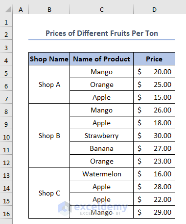
There are several methods in Excel for the calculation of the average. To do this, we have made a dataset of Prices of Different Fruits Per Ton from 3 different Shops. The dataset is like this.
We’ll now try the following seven different methods to calculate the average price.
1. Applying AVERAGE Function to Calculate Average Price in Excel
The AVERAGE function is the simplest function for calculating the average. We can use it when we need to find the direct average without any criteria. We can write the formula in cell D17 like this.
=AVERAGE(D5:D16)Here, D5:D16 is the price of fruits from cells D5 to D16.
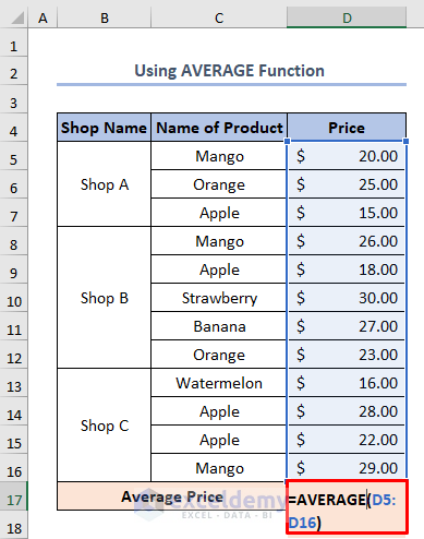
After pressing ENTER, we find the output as 23.25.

Read More: How to Calculate Average Share Price in Excel
2. Using AVERAGEA Function to Calculate Average Price
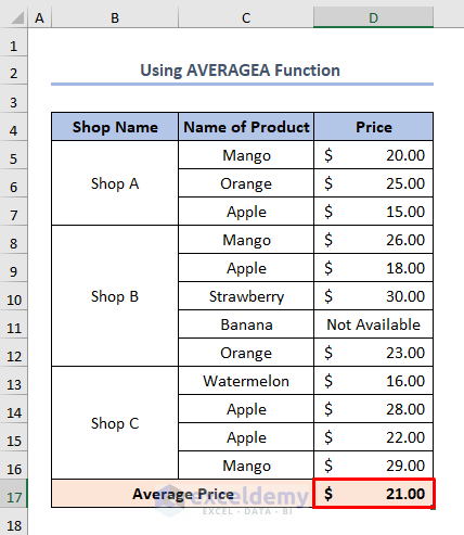
We can use the AVERAGEA function when we have text in our selected argument cells. The AVERAGEA function evaluates text as zero, logical value TRUE as 1, and logical value FALSE as zero. We have changed the Price of Banana to Not Available in Shop B to show how AVERAGEA function works. We can write the formula in the D17 cell like this.
=AVERAGEA(D5:D16)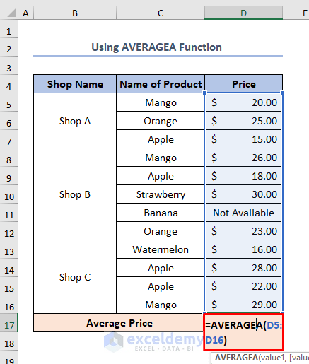
Similarly, by pressing ENTER, we find the calculated Average Price as 21.00.
3. Utilizing AVERAGEIF Function to Calculate Conditional Average Price
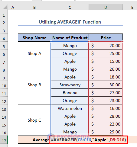
The AVERAGEIF function searches the provided range for cells that fulfill particular criteria, and then calculates the arithmetic mean of those cells. If we want to calculate the Average Price of Apples only, we can write the formula in cell D17 like this.
=AVERAGEIF(C5:C16,”Apple”,D5:D16)Here, C5:C16 refers to the Name of Products from cells C5 to C16. Apple is the criteria here, and this function will calculate the average of Apples only.
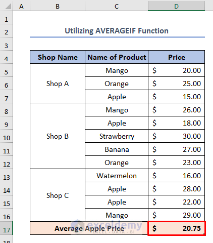
Lastly, by pressing ENTER, we find the following output as 20.75.
4. Applying SUM and COUNTA Functions
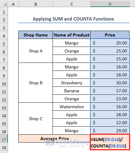
Another simple method to calculate the average is the use of the SUM and COUNTA functions. We can apply this formula to cell D17 like this.
=SUM(D5:D16)/COUNTA(D5:D16)Here, the SUM function first calculates the summation from cells D5 to D16, which we have put in the formula. The COUNTA function counts the argument number i.e. calculates how many arguments are there from cell D5 to D16. Then the output from the SUM function is divided by the output of the COUNTA function to calculate the average.
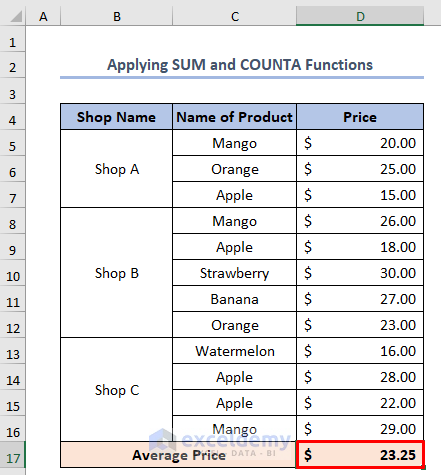
As a result. after pressing ENTER, we find the calculated Average Price is 23.25.
5. Using SUBTOTAL Function
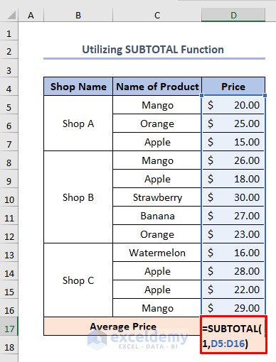
The SUBTOTAL function is extremely effective in Excel. We can use this function for various purposes. To calculate the average, we can write this formula like this.
=SUBTOTAL(1,D5:D16)After putting SUBTOTAL in the formula, we will see different function names in the string. Among them, AVERAGE is the first function. Here, 1 refers to mainly this AVERAGE function.
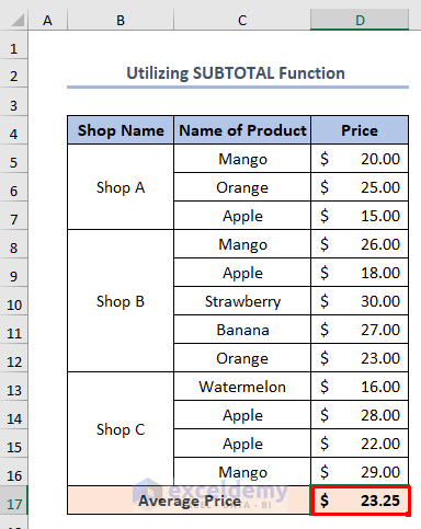
Subsequently, by clicking ENTER, we find the output as 23.25.
6. Applying AVERAGE and LARGE OR SMALL Functions
We can use either the LARGE function or the SMALL function with the AVERAGE function to calculate certain largest or smallest values’ average.
6.1 Finding Average of 3 Largest Prices
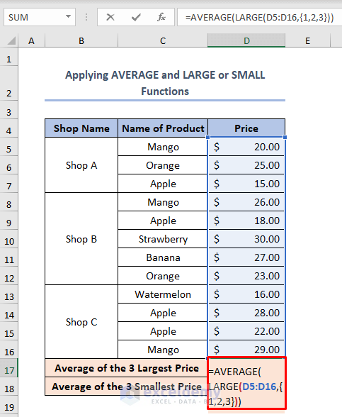
When we want to calculate the average of certain limited large values’ we need to apply the combination of AVERAGE and LARGE functions. To find the average of the three largest prices, we need to write the formula in cell D17 like this.
=AVERAGE(LARGE(D5:D16,{1,2,3}))Here, the formula LARGE(D5:D16,{1,2,3}) will first find the largest 3 values from cell D5 to D16. Then the AVERAGE function calculates the average of the outputs of the first formula.
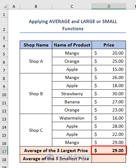
As a result, after clicking ENTER, we find the Average of the 3 Largest Price as 29.
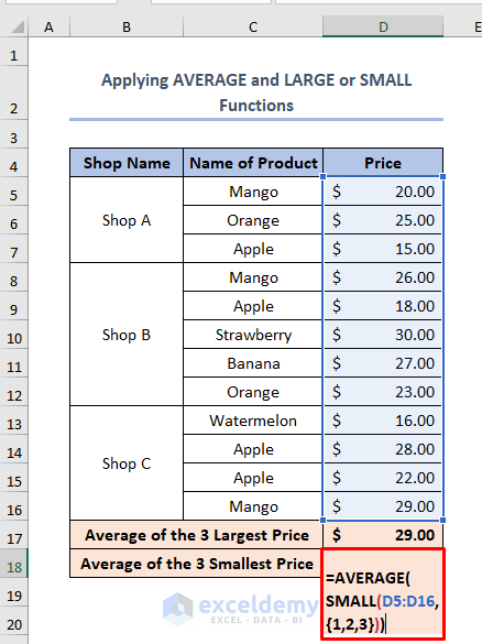
6.2 Finding Average of 3 Smallest Prices
The SMALL function works similarly to the LARGE function. We need to write the formula in the cell D18 like this.
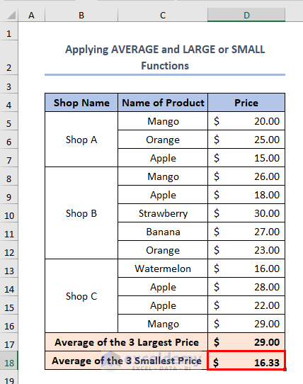
=AVERAGE(SMALL(D5:D16,{1,2,3}))Here, the formula SMALL(D5:D16,{1,2,3}) will first find the smallest 3 values from cell D5 to D16. Then the AVERAGE function calculates the average of the outputs of the formula like the previous one.
As a result, by clicking ENTER, we get the output as 16.33 like this.
7. Using SUMPRODUCT Function to Calculate Weighted Average
In a dataset, calculating weighted average is the average of numbers with variable degrees of relevance. All of the weighting variables or percentages in the below example add up to 100%. As a result, when computing the average marks, we don’t need to divide the sum of all weightage elements. All we have to do now is multiply all of the marks by their respective weightage factors and add all of the products together.
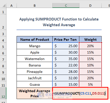
The sum of the products of related ranges or arrays is returned by the SUMPRODUCT function. In order to use this function, we must provide the range of cells in the first argument that includes all marks. All of the weighting elements will be accommodated in the second argument. So, to determine the weighted average marks, we’ll need to use the SUMPRODUCT function. We can write the formula in the C12 cell like this.
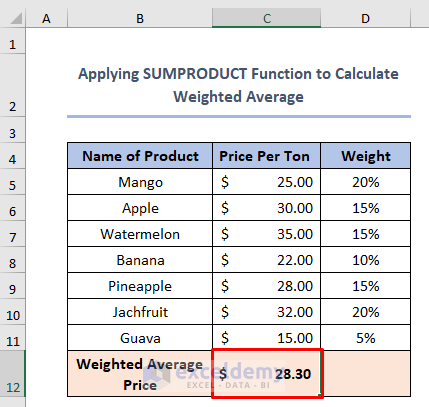
=SUMPRODUCT(C5:C11,D5:D11)Here, D5:D11 refers to the Weighting Factors of different fruits for prices in the market from cells D5 to D11.
Eventually, after pressing ENTER, we find the Weighted Average Price as 28.30.
Things to Remember
- We can use the AVERAGE function, the combination of SUM and COUNTA functions, and SUBTOTAL functions to calculate the average price directly without any conditions.
- If we need to add some conditions, we must apply the AVERAGEIF function or a combination of LARGE or SMALL functions with the AVERAGE
- Again, we can apply the AVERAGEA function if there is a mixture of values and texts in the selected cells.
Download Practice Workbook
Conclusion
In this article, we have discussed almost all of the formulas that are related to calculating the average price. We hope this article will be very beneficial for you.
Related Articles
- Average Attendance Formula in Excel
- How to Calculate Average, Minimum And Maximum in Excel
- How to Calculate Average of Averages in Excel
- How to Calculate Average True Range in Excel
- How to Calculate Average Percentage in Excel
- How to Calculate Average Percentage of Marks in Excel
- How to Calculate Class Average in Excel
- How to Calculate Average Revenue in Excel
- How to Calculate Average Quarterly Revenue in Excel
- How to Calculate Average Length of Stay in Excel
<< Go Back to Excel Average Formula Examples | How to Calculate Average in Excel | How to Calculate in Excel | Learn Excel
Get FREE Advanced Excel Exercises with Solutions!
