Generic Formula to Calculate the Average True Range
The stock’s daily high, daily low, and daily close price are needed to calculate the average true range.
To consider the closing price of the previous day:
It chooses the maximum among the three differences:
- The present high minus the present low
- The absolute value of the present high minus the previous close
- The absolute value of the present low minus the previous close
The calculation of the average true range for the first period is:
Welles proposed using a smoothed average of 14 days. So, in the above formula, n equals 14. The average of the true range is calculated for the first 14 days, and from that result, the first average true range is returned. The next ATRs will be calculated using an exponential moving average with the following formula:
ATRt is the present average true range.
ATRt-1 is the previous average true range.
n represents 14 (for a 14-day moving average).
TRt is the present true range.
The standard value of n is 14, as the average volatility over the previous 14 days is shown by ATR.
Read More: How to Calculate 7 Day Moving Average in Excel
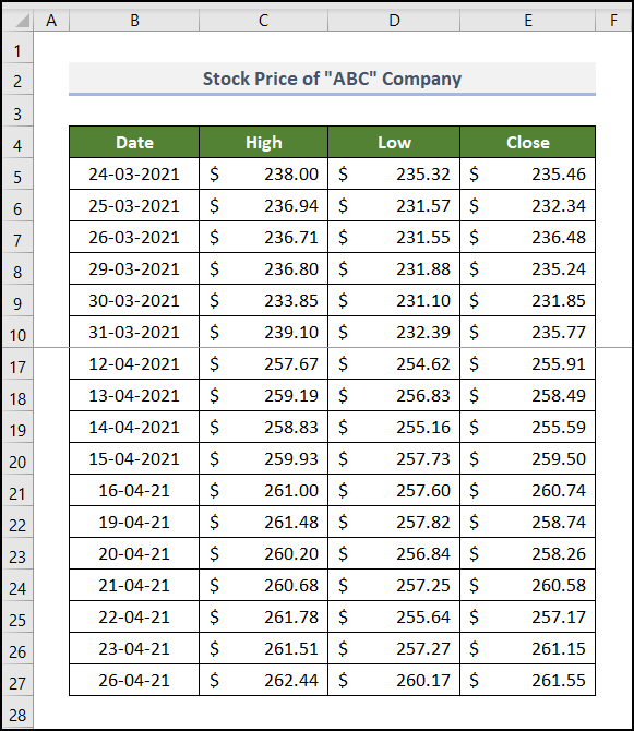
This dataset showcases a report on the Stock Price of the “ABC” Company. It includes the High, Low, and Close prices of stock from 24 March 2021 to 26 April 2021. Freeze Panes was used.
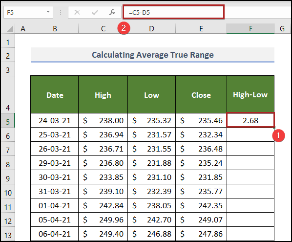
Step1 – Determine the Present High Minus the Present Low
Steps:
- Select F5 and enter the following formula.
=C5-D5
C5 and D5 represent the High and Low prices of the corresponding day.
- Press ENTER.
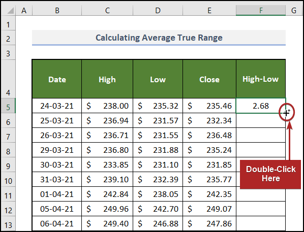
- At the bottom-right corner of F5, the cursor will display a plus (+) sign. It’s the Fill Handle tool. Double-click it.
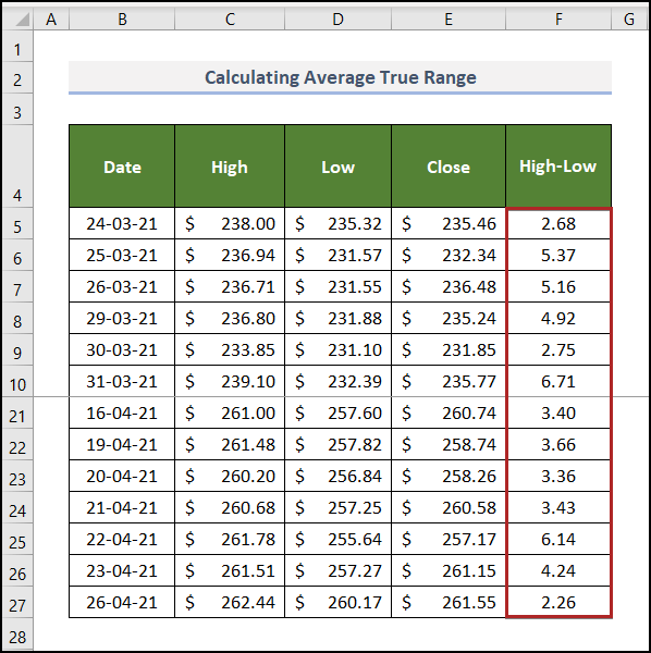
This is the output.
Read More: How to Get Average Time in Excel
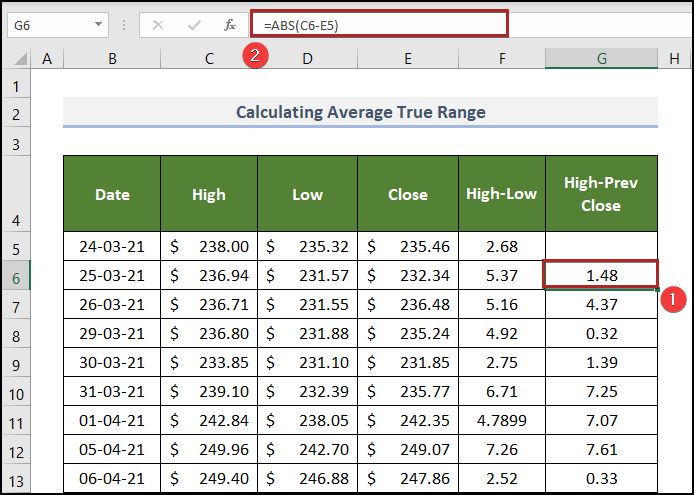
Step 2 – Calculate the Present High Minus the Previous Close
Steps:
- Select G6 and enter the following formula.
=ABS(C6-E5)
C6 and E5 represent the present high price and the previous close price. The ABS function returns the absolute value of their difference. It always returns a positive value.
- Press ENTER.
Read More: How to Calculate Average, Minimum And Maximum in Excel
Step 3 – Compute the Present Low Minus the Previous Close
Steps:
- Select H6 and enter the following formula.
=ABS(D6-E5)
- Press ENTER.
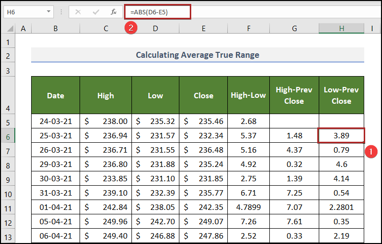
Here, cells G5 and H5 are blank because there is no previous day before these days.
Read More: How to Calculate Monthly Average from Daily Data in Excel
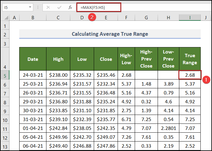
Step 4 – Calculate the True Range
Steps:
- Select I5 and enter the following formula.
=MAX(F5:H5)
F5:H5 represents values of high-low, high-previous close, and low-previous close.
The MAX function returns the maximum value among data in F5:H5.
- Press ENTER.
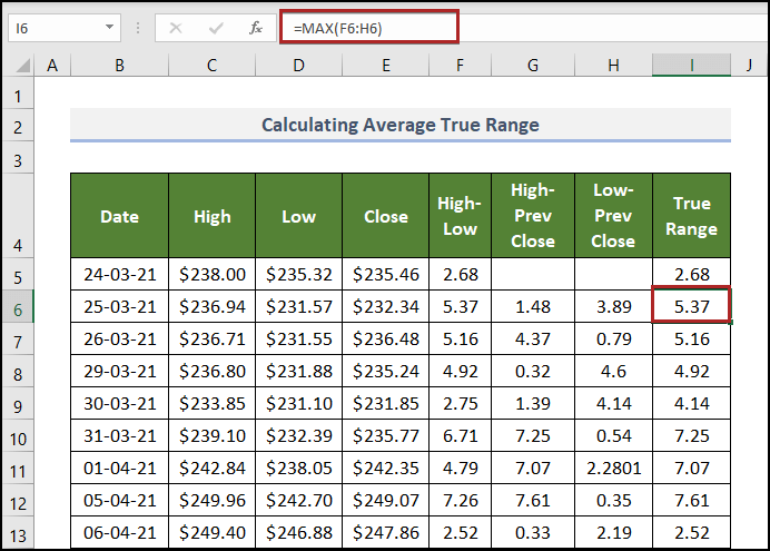
Check if the formula returns the correct answer in I6 . 5.37, 1.48, and 3.89 are displayed in F6, G6, and H6.
5.37 is the greatest value. The function also returns this value.
Read More: How to Calculate Average of Multiple Ranges in Excel
Step 5 – Calculate the Average True Range
Steps:
- Select J18 and enter the following formula.
=AVERAGE(I5:I18)
The AVERAGE function returns the arithmetic mean of the arguments.
- Press ENTER.
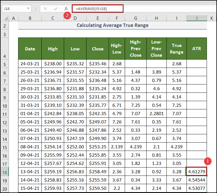
J5:J17 was kept blank.
Go back to the generic formula: the ATR for the first period is calculated using the arithmetic mean of consecutive 14 days. 14 days of data were stored in cells I5:I18.
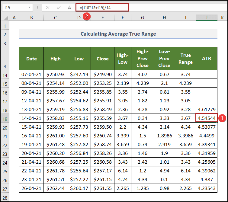
To determine the ATR for the following days:
- Select J19 and enter the following formula.
=(J18*13+I19)/14
The formula is explained in the previous section.
- Press ENTER.
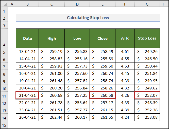
How to Calculate ATR Stop Loss
ATR can assist you in determining where to set your stop loss.
Below is a part of the previous dataset with calculated ATR values.
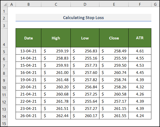
The second multiple of the ATR value was used here. Calculate the stop loss for each date:
Steps:
- Create a new column: Stop Loss.
- Select G5 and enter the following formula.
=E5-2*F5
- Press ENTER.
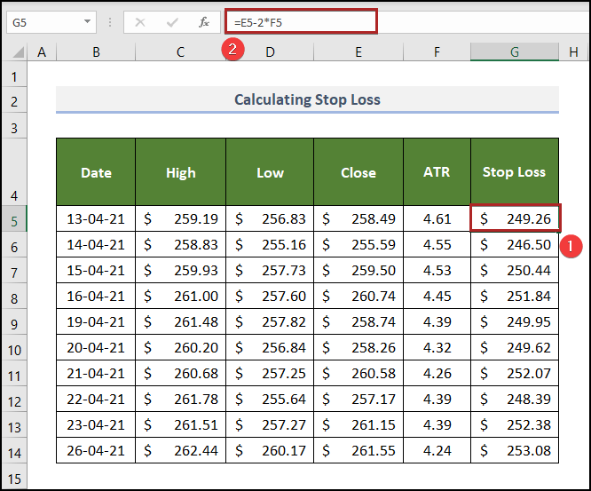
You purchased stock on 13 April 2021 at the close price: $258.49.
You set a stop loss at $249.26: if the price of this stock falls on this, you won’t take any further risk and sell it.
If you buy it on 21 April at a price of $260.58, you will set the stop loss at $252.07.
Read More: How to Calculate Average of Multiple Columns in Excel
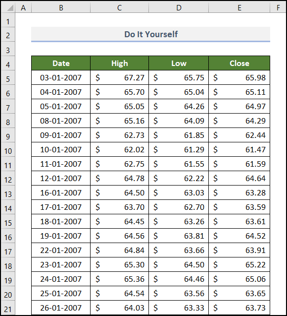
Practice Section
Practice here.
Download the following Excel workbook.
Related Articles
- Average Attendance Formula in Excel
- How to Calculate Average of Averages in Excel
- How to Calculate Average Percentage in Excel
- How to Calculate Average Percentage of Marks in Excel
- How to Calculate Class Average in Excel
- How to Calculate Average Revenue in Excel
- How to Calculate Average Quarterly Revenue in Excel
- How to Calculate Average Share Price in Excel
- How to Calculate Average Length of Stay in Excel
- How to Calculate Average Price in Excel
<< Go Back to Excel Average Formula Examples | How to Calculate Average in Excel | How to Calculate in Excel | Learn Excel
Get FREE Advanced Excel Exercises with Solutions!
