How to Calculate 7 Day Moving Average in Excel (4 Ways)

What Is the Moving Average?

The moving average is a type of average of numbers where the time frame remains the same but the data keeps updating as new data is added.

For example, we have a list of the daily arriving customer numbers of a shop. To get the average customer number, we generally sum up the total number of customers for 7 days and then divide the sum by 7. This is the general average calculation concept.

In the case of moving average or running average, the days continue, and the number of customers keeps updating. As a result, the moving average changes too. It’s not a static value now.

Types of the Moving Average

The moving average can be divided into 3 major types. Those are,

Simple Moving Average
Weighted Moving Average
Exponential Moving Average

Simple Moving Average: When you calculate the average data of a certain numerical value by summing them up first and then dividing, it’s called Simple Moving Average. You can calculate the Simple Moving Average in Excel using the AVERAGE function, or the SUM function.

Weighted Moving Average: Suppose, you want to forecast the average temperature. It is possible that the latest data can predict better than the old data. In that case, we put more weight on the recent data. Thus, calculating the moving average with weights is called the Weighted Moving Average.

Exponential Moving Average: The Exponential Moving Average is a type of moving average where more weights are given to the recent data and fewer weights for the older data.

How to Calculate a 7-Day Moving Average in Excel: 4 Ways

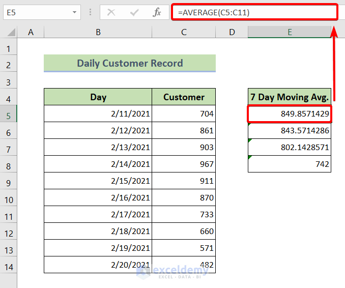
Method 1 – Use the AVERAGE Function to Calculate the 7-Day Simple Moving Average in Excel

Insert the AVERAGE function in a cell to collate the first seven values.

=AVERAGE(C5:C11)

Hit Enter.
Drag down the Fill Handle. This moves the cell reference and recalculates the average for subsequent days.

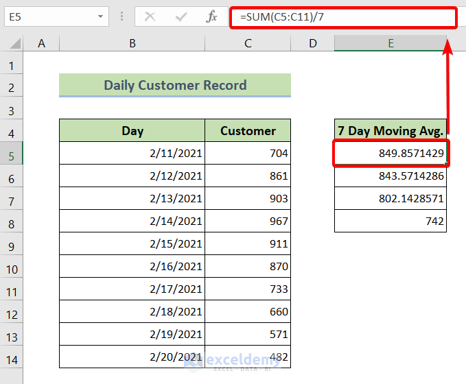
Method 2 – Calculate the 7-Day Simple Moving Average in Excel Using the SUM Function

Insert the following formula for the first result (first seven days).

=SUM(C5:C11)/7

Hit Enter.
Drag down the Fill Handle tool to the other cells to calculate the moving average.

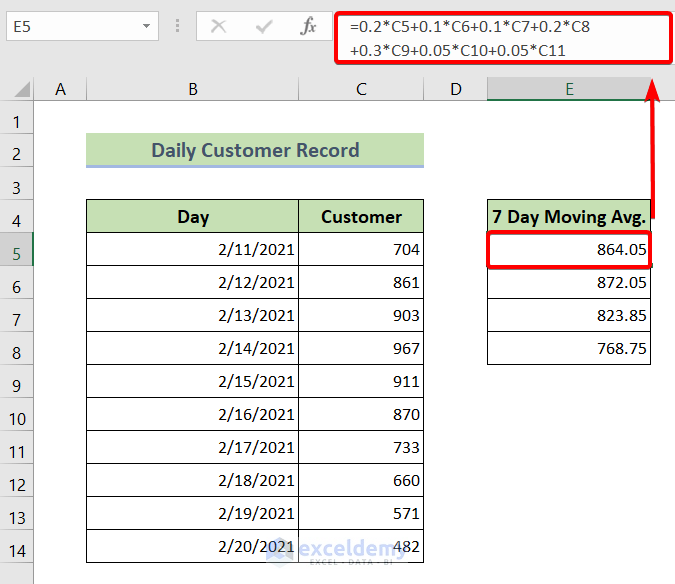
Method 3 – Find the 7-Day Weighted Moving Average in Excel

We have the following weights for the 7-day moving average formula: 0.2, 0.1, 0.1, 0.2, 0.3, 0.05, and 0.05, for each day respectively. The weights must add up to 1.

Enter the following formula for the Weighted Moving Average in cell E5.

=0.2*C5+0.1*C6+0.1*C7+0.2*C8 +0.3*C9+0.05*C10+0.05*C11

Hit Enter.
Drag down the Fill Handle.

Method 4 – Calculate the 7-Day Exponential Moving Average in Excel

The general formula to calculate the 7-day Exponential Moving Average (EMA) in Excel is:

EMA = [Recent Value - Last EMA] * (2 / N+1) + Last EMA

In the formula above, you can insert any value for the N (number of days) as per your recruitment.

Enter the following formula in cell E5 to copy the first value of the data.

=C5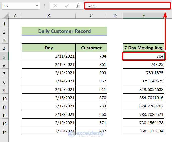

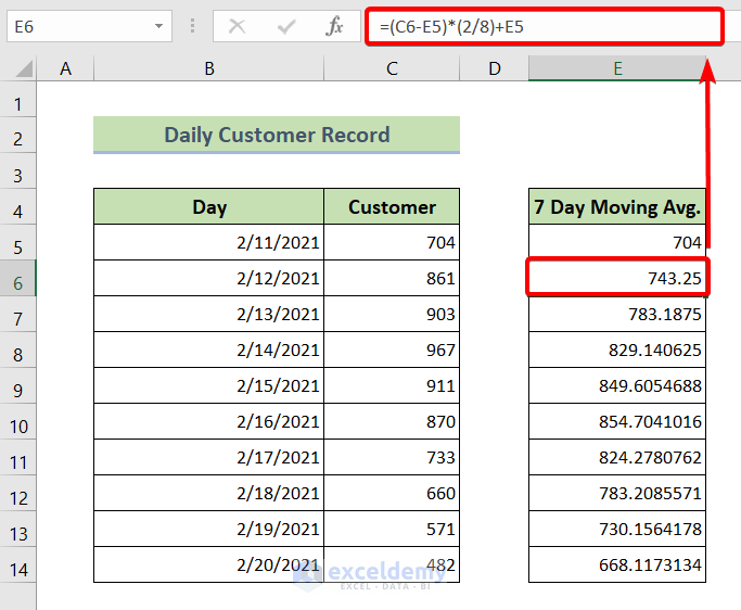
Use the following formula in cell E6.

=(C6-E5)*(2/8)+E5

Hit Enter and drag down the Fill Handle.

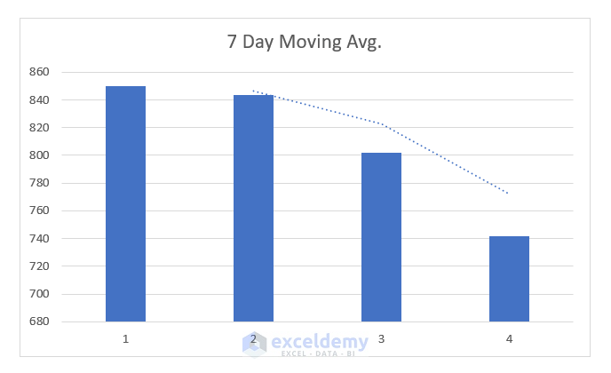
Insert a Moving Average Chart in Excel

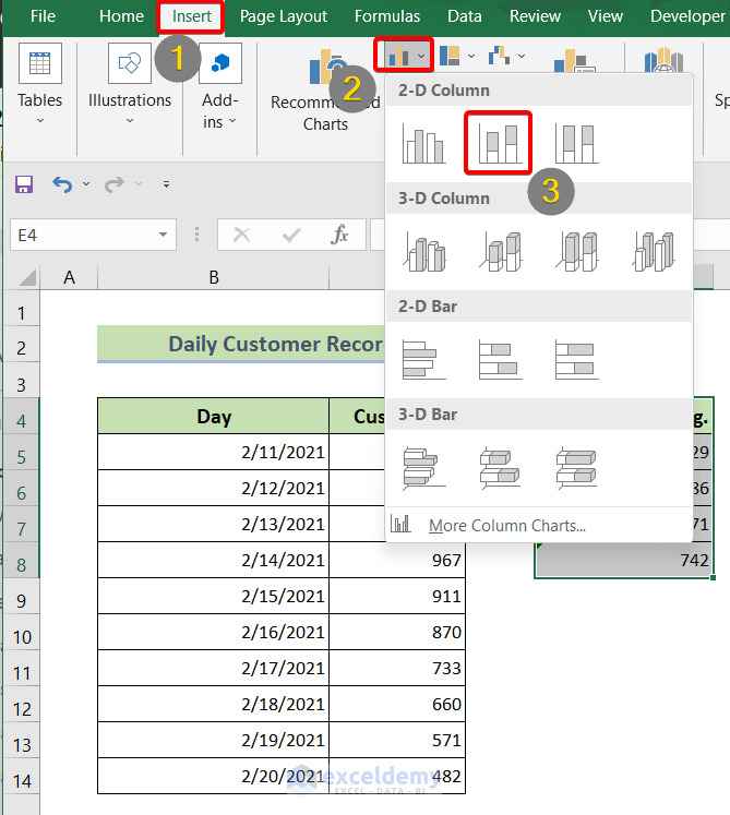
Select the moving average values first.
Go to the Insert tab.
Insert a Clustered Column 2-D chart.

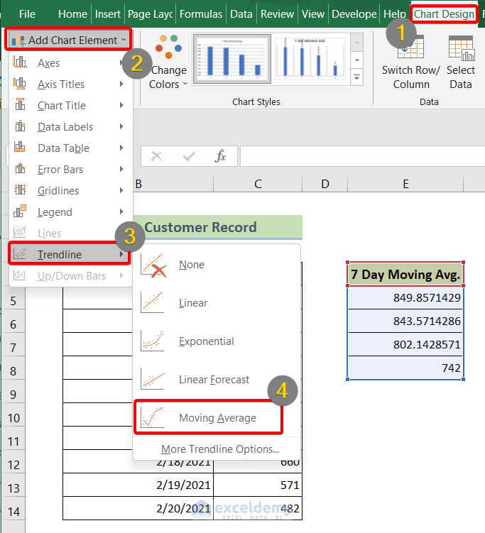
Click on the 2-D chart and go to the Chart Design tab.
Navigate to the Add Chart Element.
From the drop-down menu, choose Trendline.
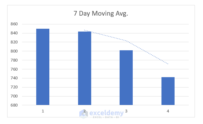
Under the Trendline, you will find the Moving Average. Click on it to apply.