What is the Moving Average?
The Moving Average is the change in the average of a data series overtime.
If you need to provide the moving average of the sales value on day 3, you have to consider the sales value of Days 1, 2, and 3. And to provide the moving average of the sales value on day 4, you have to consider the sales value of days 2, 3, and 4. As new data is added, you must keep the time period/ interval (3 days) the same, using the added data to calculate the moving average.
The moving average smooths irregularities (peaks and valleys) and recognize trends. The larger the interval is to calculate the moving average, the more the smoothing occurs, as more data points are included.
The OFFSET function is used to calculate the moving average.
The combined formula of the AVERAGE function and the OFFSET function is:
=AVERAGE(OFFSET(A1, 0, 0, -n, 1))- A1 = reference
- n = the number of spans to include in each average
The OFFSET function returns a range that is passed into the AVERAGE function to extract the Moving Average.
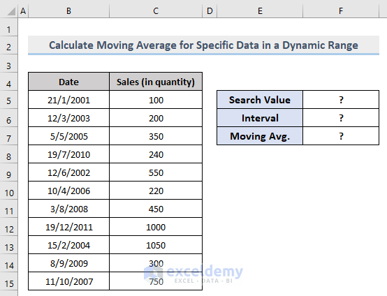
Example 1 – Calculate the Moving Average for Specific Data in a Dynamic Range
The sample dataset showcases Date and Sales.
To find the moving average for each date:
Steps:
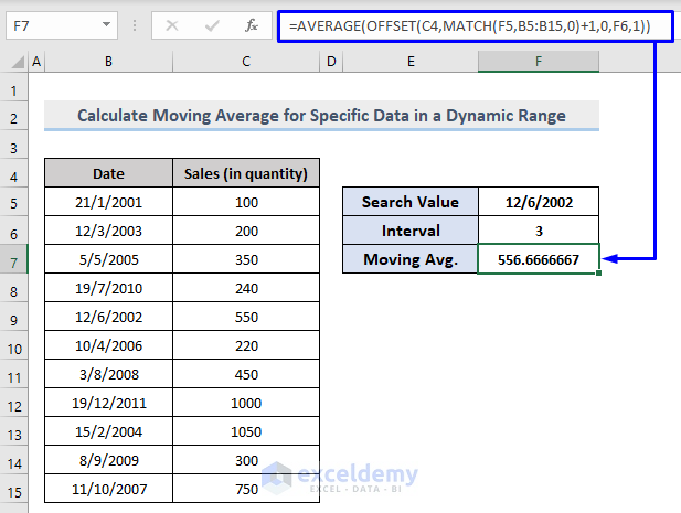
- In F7, use the following formula:
=AVERAGE(OFFSET(C4,MATCH(F5,B5:B15,0)+1,0,F6,1))- C4 = Starting point, Column header.
- F5 = Search value to extract the moving average (here, 12/6/2002).
- B5:B15 = Search range to search the match for the search value.
- F6 = The interval (here, 3).
- Press Enter. You will get the moving average for the given interval.
Observe the GIF.
If you change the intervals, F7 will automatically be updated according to the input value.
You can also change the Search Value to extract the data for specific dates. The result in F7 will show the corresponding moving average.
Observe the GIF below.
Formula Breakdown
- MATCH(F5,B5:B15,0)
- Result: 5
- Description: The MATCH function returns the position of lookup value in the search range/ array. The syntax for the MATCH function is:
=MATCH(lookup_value, array, [match_type])
-
-
- F5 = lookup_value
- B5:B15 = array
- 0 = [match_type], exact match
-
It counts the position of the search value 12/6/2002 in B5:B15 and finds its position: 5.
- OFFSET(C4,MATCH(F5,B5:B15,0)+1,0,F6,1) -> becomes:
- OFFSET(C4,5+1,0,F6,1)
- Result: 220, 450, 1000
- Description: The OFFSET function takes the cell reference C4 (1st argument) as the starting point.
- Not to include the selected date, +1 was added to the MATCH function. It instructs the formula to find the selected date and go down one cell.
- To stay in the same column, it was set to 0.
- Height, F6 depends on the condition. To include the selected date, the cell reference must be used in the calculation.
- The width is set to 1.
- AVERAGE(OFFSET(C4,MATCH(F5,B5:B15,0)+1,0,F6,1)) -> becomes:
- AVERAGE(220, 450, 1000)
- Result: 556.6666667
- Description: The average result of 220, 450, 1000
Read More: How to Calculate 7-Day Moving Average in Excel
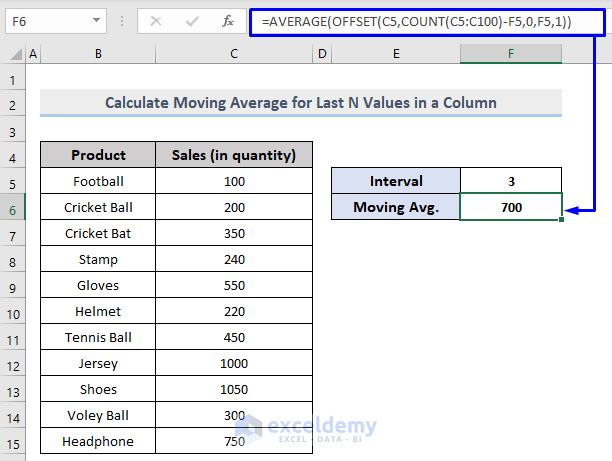
Example 2 – Get the Rolling Average for the Last N-th Values in a Dynamic Column in Excel
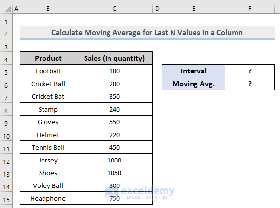
The formula is:
- N = the number of values to include to calculate the average
- To calculate the moving average, use the formula:
=AVERAGE(OFFSET(C5,COUNT(C5:C100)-F5,0,F5,1))- C5 = Start point of the range
- F5 = The interval (3).
It will return the moving average of the last 3 values in a dynamic column.
Observe the GIF.
If you change the intervals, F6 will automatically be updated according to the input value.
Formula Breakdown
- COUNT(C5:C100)
- Result: 11
- Description: The COUNT function counts the values in Column C. C5 is the starting point of the range to calculate.
- OFFSET(C5,COUNT(C5:C100)-F5,0,F5,1) -> becomes:
- OFFSET(C5,11-3,0,3,1)
- Result: 1050, 300, 750
- Description: The OFFSET function takes the cell reference C5 (1st argument) as the starting point, and calculates the value returned by the COUNT function moving 3 rows up (-3 in the 2nd argument). It returns the sum of values in a range consisting of 3 rows (3 in the 4th argument) and 1 column (1 in the last argument): the last 3 values you want to calculate.
- AVERAGE(OFFSET(C5,COUNT(C5:C100)-F5,0,F5,1)) -> becomes:
- AVERAGE(1050, 300, 750)
- Result: 700
- Description: The AVERAGE function calculates the returned sum values to extract the moving average.
Read More: How to Calculate Exponential Moving Average in Excel
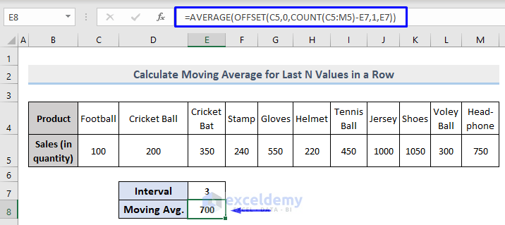
Example 3 – Extract the Moving Average for the Last N-th Values in a Dynamic Row in Excel
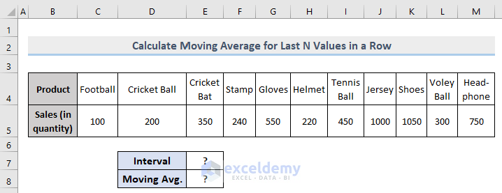
The formula is very similar to the one used in Example 2, but instead of the entire range, there is a fixed range.
=AVERAGE(OFFSET(C5,0,COUNT(C5:M5)-E7,0,E7,1))- C5 = Start point of the range
- M5 = Endpoint of the range
- E7 = The interval (3).
It will return the moving average of the last 3 values in a dynamic row.
Observe the GIF.
If you change the intervals, E8 will automatically be updated according to the input value.
Read More: How to Average Every Nth Row in Excel
Download Workbook
Download the free practice Excel workbook.
Related Articles
- How to Calculate Running Average in Excel
- How to Generate Moving Average in Excel Chart
- How to Calculate Centered Moving Average in Excel
<< Go Back to Moving Average | Calculate Average in Excel | How to Calculate in Excel | Learn Excel
Get FREE Advanced Excel Exercises with Solutions!

Hello Sanjida,
How do you compute a running maximum of values in a given column using dynamic arrays
as in the following example
values running maximum
113.4200 113.42000
109.5806 109.58065
104.5533 104.55333
103.2129 103.21290
102.0600 102.68667
102.5710 102.68667
102.6867 102.68667
102.4419 102.53333
102.5333 102.53333
101.6419 101.64194
101.1800 101.18000
Best regards!
gianluca
Hello Gianluca,
Hope you are doing well. Thank you for your query. Well, I can see two columns here and you need to get the running maximum of the values using a dynamic array. Therefore, you can use the MAX function to get the running maximum from the dataset. You may follow the below image to use the MAX function as an array function. If you use the total column in the formula as below then the formula will work like an array formula. You can add or change any value within the range and the running maximum value will change according to your dataset.
[wpsm_box type="green" float="none" textalign="center"]
=MAX($B:$B,$C:$C)[/wpsm_box]
Here, if add another column then the formula adds the values in the range and changes the output as below.