Moving Average Formula in Excel (8 Uses with Examples)

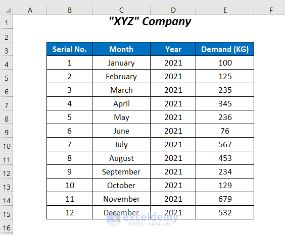
In the dataset below, we have some records of the Demand of a company for the 12 months of the year 2021. Using these values we will calculate the moving average and forecast the demand for January 2022. We will demonstrate a 3-point moving average, so we will require 3 values for our calculations.

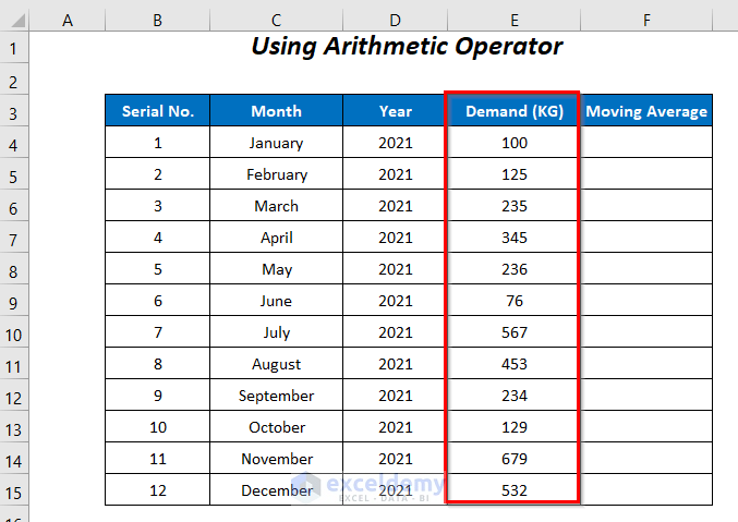
Method 1 – Using Arithmetic Operators

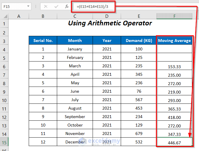
We can use the arithmetic operator “+” to calculate the moving average and forecast the demand for January 2022.

Steps:

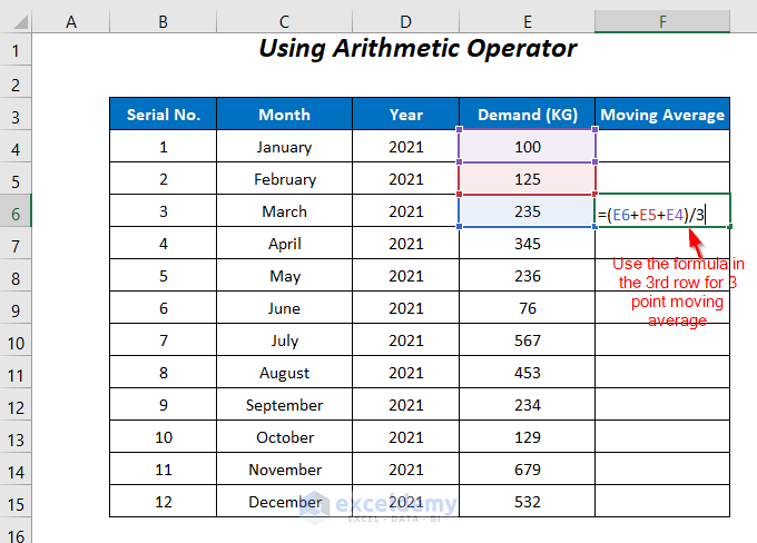
• Select a cell in the 3rd row of the dataset.

As we are using 3 point moving average and as this average requires at least 3 values, if we used a cell in the first two rows then we wouldn’t have enough values.

• Enter the following formula in cell F6:

E6, E5, and E4 are the first 3 values. We calculate the average by summing them and then dividing the result by 3.

• Press ENTER and drag down the Fill Handle tool.

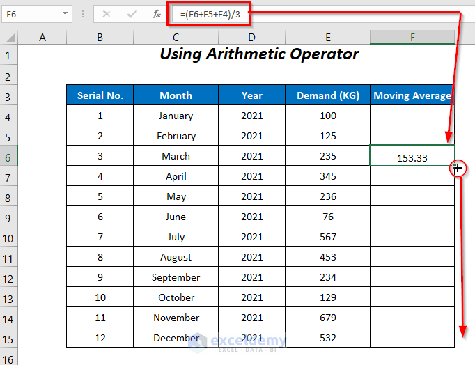
The moving averages are calculated.

Read More: How to Calculate Running Average in Excel

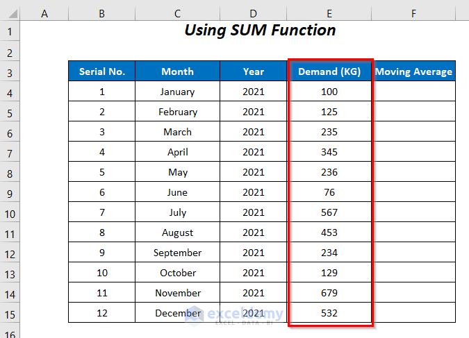
Method 2 – Using the SUM Function

We can alternatively use the SUM function to perform the same task as the previous method.

Steps:

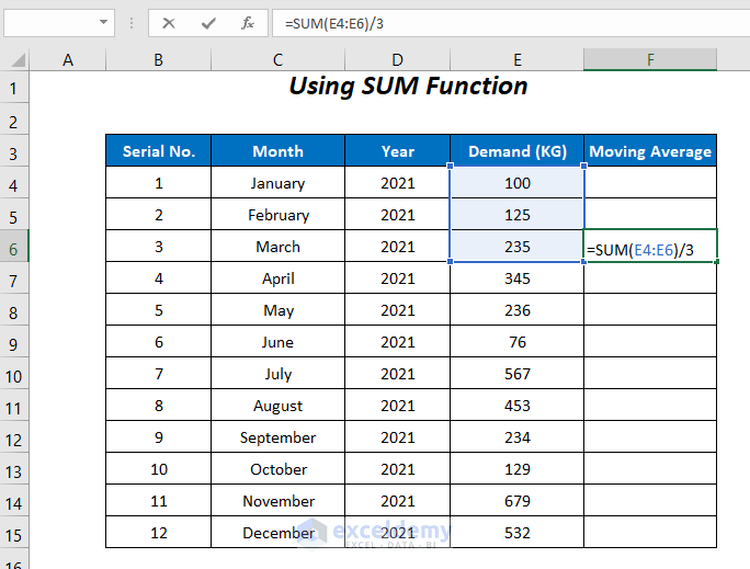
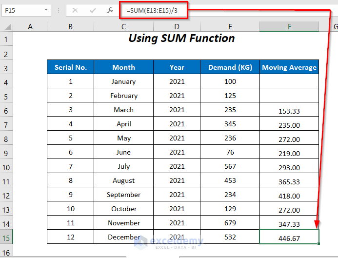
• Enter the following formula in cell F6:

SUM adds the values of the cells E6, E5, and E4, which are then divided by 3.

• Press ENTER and drag down the Fill Handle tool.

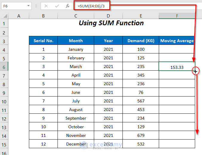
The moving averages are calculated, and the moving average in the last cell forecasts the demand for January 2022.

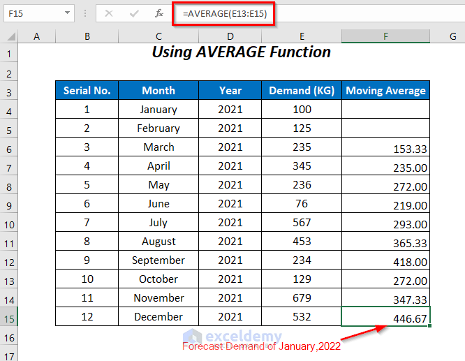
Method 3 – Using the AVERAGE Function

We can also use the AVERAGE function to determine the 3-point average of the demand.

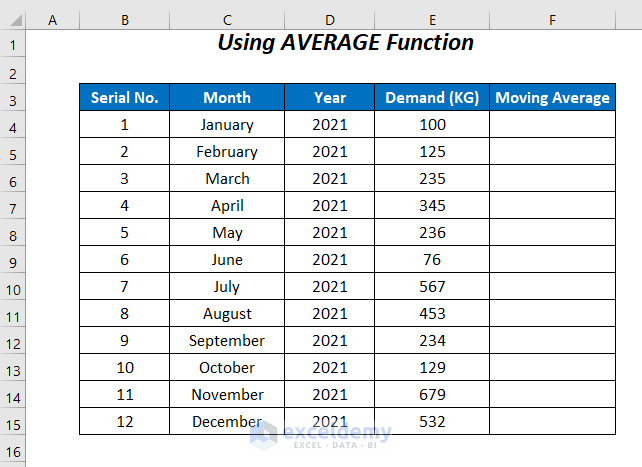
Steps:

• Enter the following formula in cell F6:

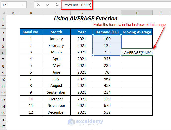
• Press ENTER and drag down the Fill Handle tool.

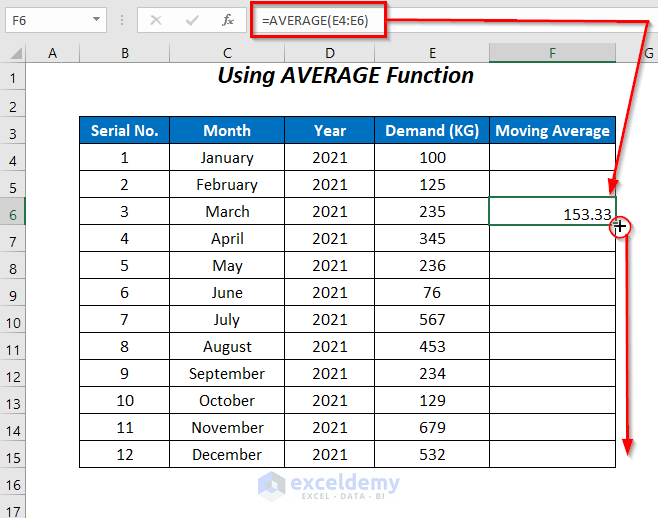
The averages for all of the remaining cells are returned, and we can forecast the demand for January 2022.

Read More: How to Calculate Centered Moving Average in Excel

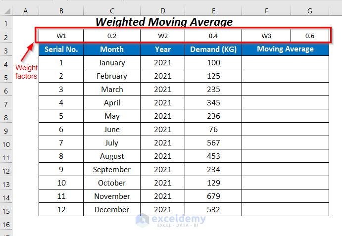
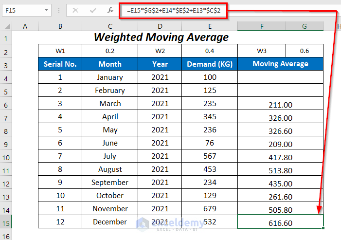
Method 4 – Formula for Weighted Moving Average

The Weighted Moving Average includes some weighted factors which will be multiplied by the values depending on their importance. As the latest demand value has more significance than the oldest demand values, we will multiply the latest value with a factor of 0.6, the second latest value by 0.4, and the oldest value by 0.2.

Steps:

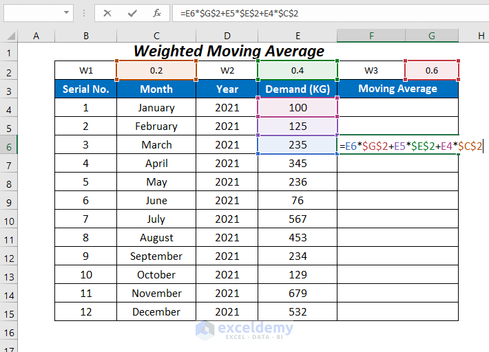
• Enter the following formula in the third row of the Moving Average column:

Here, E6 is the latest demand value in March 2021, $G$2 is the weight factor 0.6 to multiply with the value in E6, E5 is the 2nd latest demand in February 2021, $E$2 is the weight factor 0.4 to multiply with the value in E5, E4 is the oldest demand in January 2021, and $C$2 is the weight factor 0.2 to multiply with the value in E4.

• Press ENTER and drag down the Fill Handle tool.

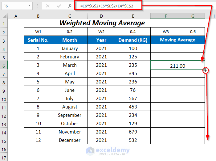
The averages for the rest of the cells are returned, and the average in the last cell will determine the demand value for January 2022.

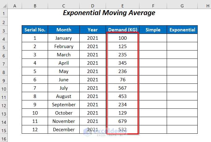
Method 5 – Formula for an Exponential Moving Average

Exponential Moving Average is another version of the Weighted Moving Average, where more weight will be given to the newest data, and the average values will decrease exponentially from the latest to the oldest data.

Steps:

• Calculate the Simple Moving Average values by following Method 3 and using the following formula:

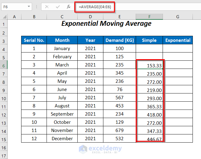
We need the actual demand value and the Simple Moving Average value for the time period immediately before the period for which we are calculating the Exponential Moving Average.

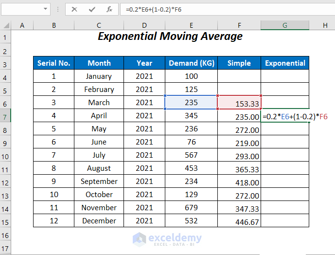
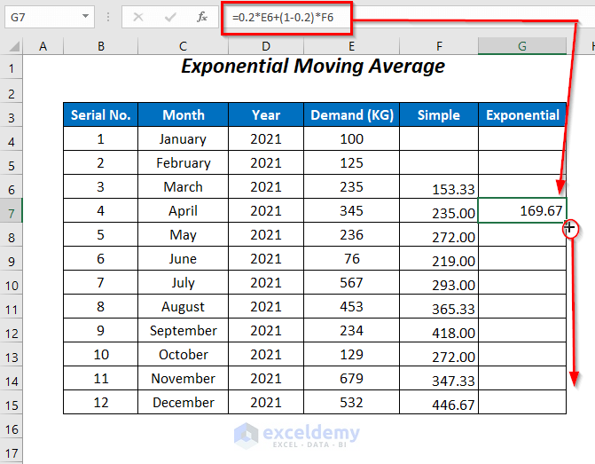
• Enter the formula below in cell G7:

Since we are using this formula to calculate the Exponential Moving Average for April 2021, we use E6, or the actual demand value for March 2021, and F6, or the Simple Moving Average value for March 2021, in the formula. 0.2 is the Smoothing factor which varies from 0.1 – 0.3.

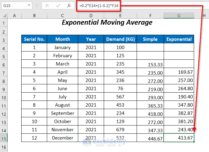
• Press ENTER and drag down the Fill Handle tool.

The averages for the rest of the cells are returned, and using the value in the last cell we forecast the demand value for January 2022.

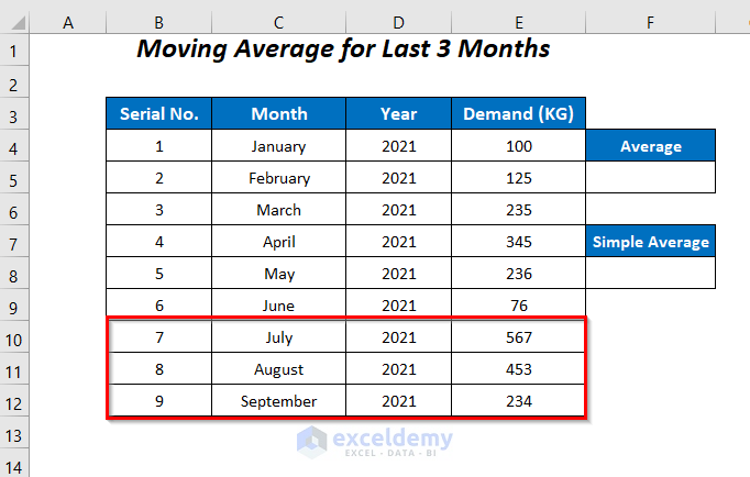
Method 6 – Formula for Last 3 Months’ Average

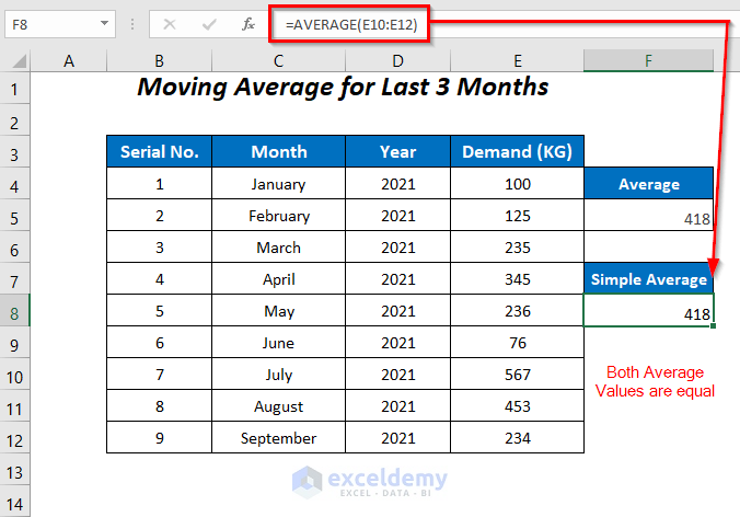
In this method, every time we enter the latest 3 months’ demand values, the average of these values is calculated automatically. To accomplish this, we use the AVERAGE, OFFSET, and COUNT functions.

Steps:

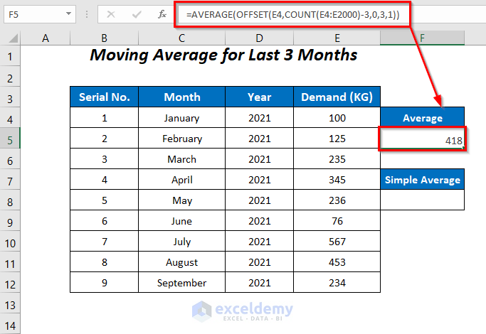
Enter the following formula in cell F5:

E4 is the cell from which it will start moving downwards and E2000 is the limit of the range. Change this number as required for your use-case. COUNT(E4:E2000)-3 is the number of rows it will move downward, 0 is the number of columns it moves to the right, the third argument 3 is the number of rows, and the fourth argument 1 is the number of columns from which the values will be extracted.

• To check the correctness of this value, enter the following formula in cell F8:

The average of the demands from July to September is equal in both cases.

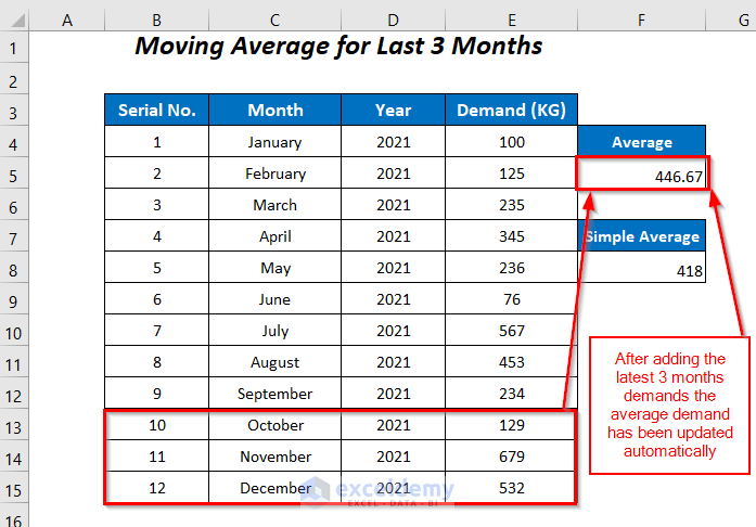
• Update the dataset with the demand values of October, November, and December.

The average value in cell F5 changes to 446.67.

• To check this value, manually change the reference of the following formula in cell F8:

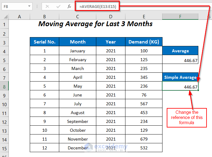
In this case too, the two average values are identical.

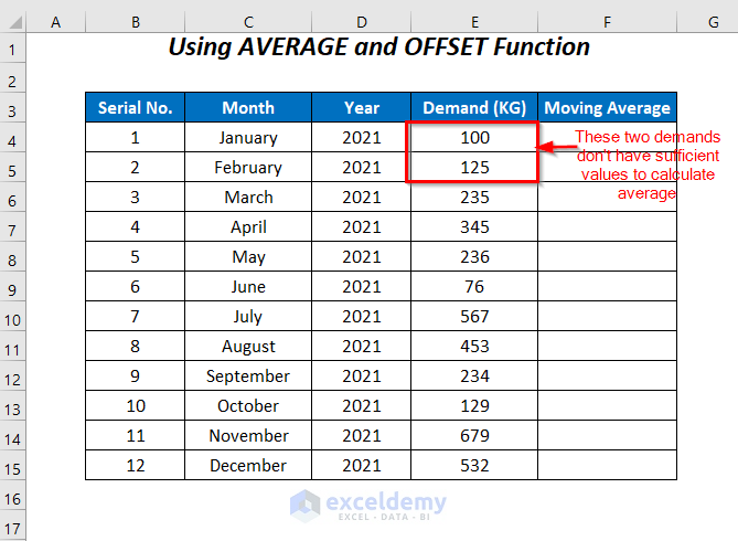
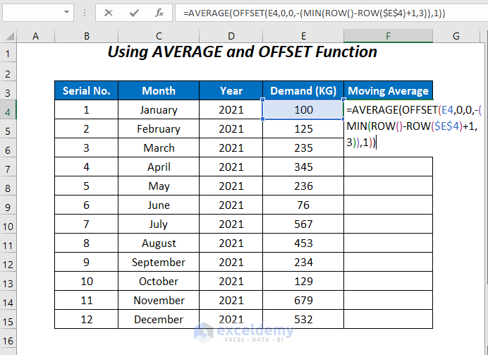
Method 7 – Simple Moving Average for Incomplete Data Using OFFSET and AVERAGE

In the previous cases, we started calculating the moving average from the 3rd row due to insufficient data in the first two rows. To solve this problem we will use a formula with the AVERAGE, OFFSET, MIN, and ROW functions.

Steps:

Enter the following formula in cell F4:

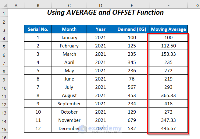
• Press ENTER and drag down the Fill Handle tool.

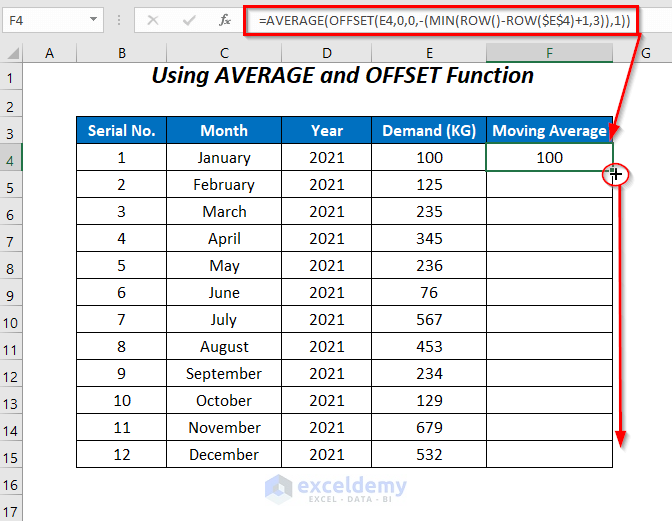
The Simple Moving Average values for all of the cells are returned.

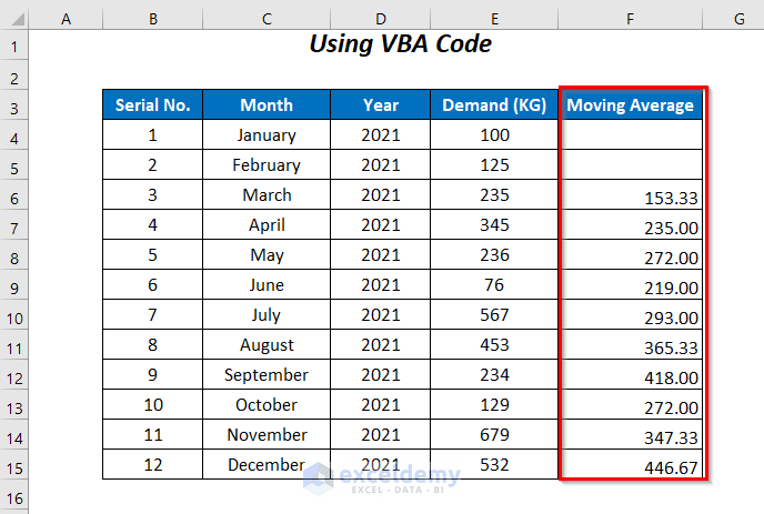
Method 8 – Using VBA Code for Simple Moving Average

We’ll use the same dataset as before.

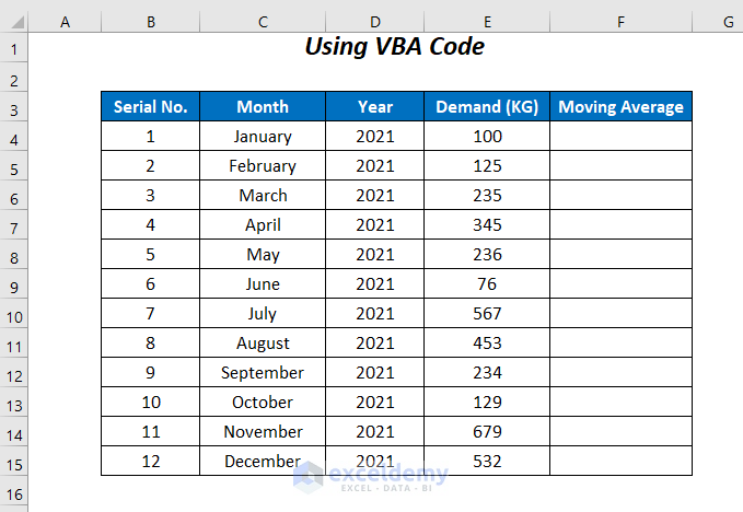
Steps:

• Go to the Developer Tab >> Visual Basic Option.

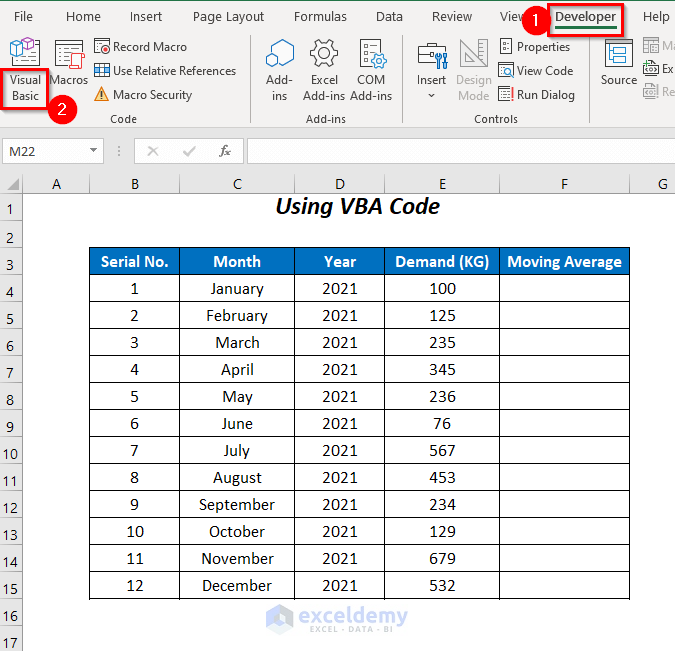
The Visual Basic Editor will open up.

• Go to the Insert Tab >> Module Option.

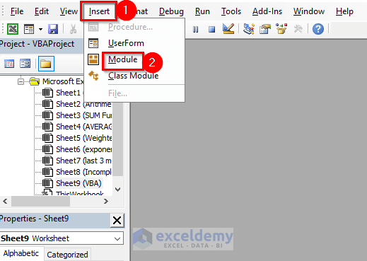
A Module will be created.

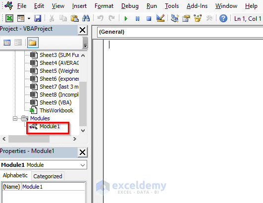
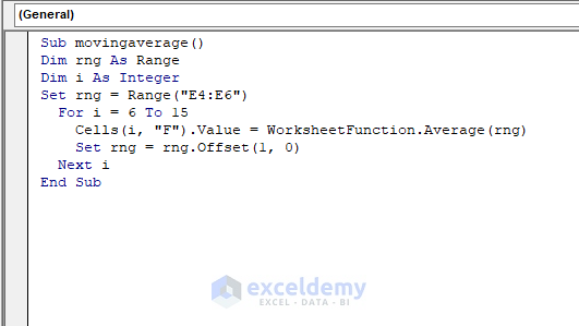
• Enter the following code in the module window:

Sub movingaverage()

Dim rng As Range
Dim i As Integer
Set rng = Range("E4:E6")

  For i = 6 To 15
    Cells(i, "F").Value = WorksheetFunction.Average(rng)
    Set rng = rng.Offset(1, 0)
  Next i

End Sub

We set the range “E4:E6” as rng. A FOR Next loop works through rows 6 to 15 calculating the moving averages, and the output values will appear in column F in the corresponding rows. Then a new range one row down from each cell will be set again with rng in each loop iteration.

• Press F5 to run the code.

The following moving averages are returned:

Read More: Calculate Moving Average for Dynamic Range

Comparing the Actual Demand Values and Moving Averages

Let’s compare the Actual Demand, Simple Moving Average, Weighted Moving Average, and Exponential Moving Average by representing the values obtained from the previous methods, and through a graph for pictorial representation.

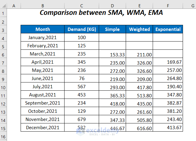
If we plot the values to visualize via a line chart:

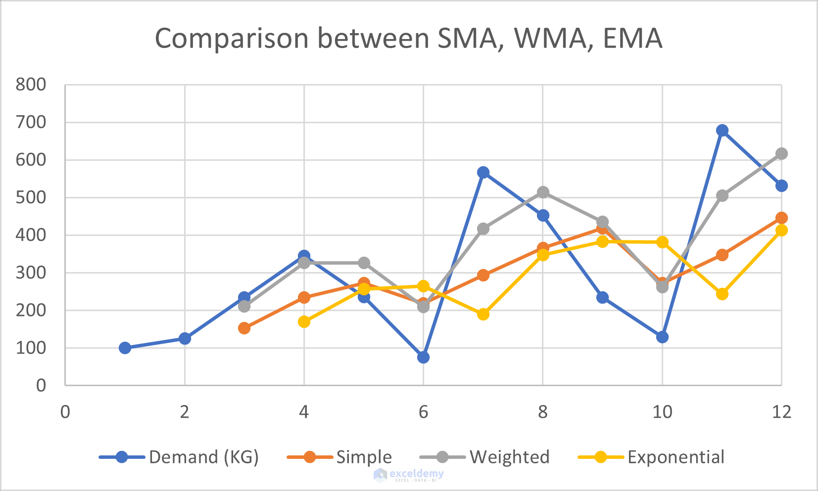
The Weighted Moving Average (WMA) is quite close to the Actual Demand, and the Simple Moving Average (SMA) and Exponential Moving Average (EMA) are near to each other.

Download the Workbook

Moving Average in Excel: Knowledge Hub

• Calculate 7 Day Moving Average in Excel
• Generate Moving Average in Excel Chart

<< Go Back to Calculate Average in Excel | How to Calculate in Excel | Learn Excel