Method 1 – Calculating Weekly Average from Daily Data
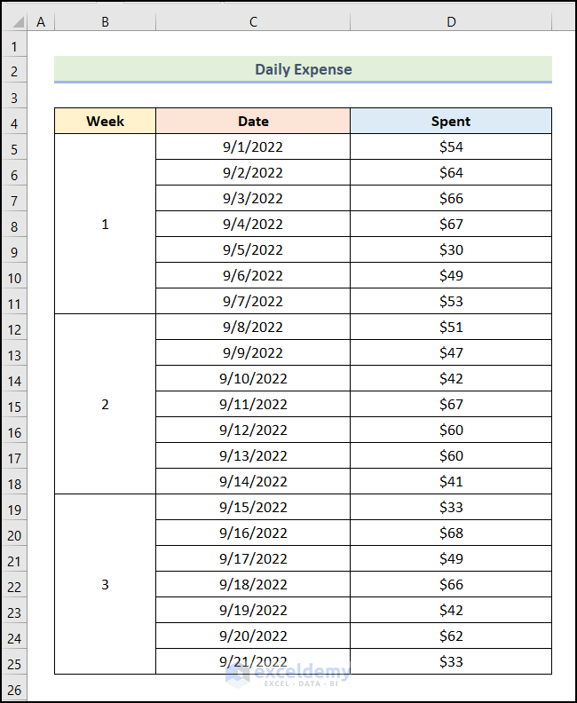
In the dataset, Daily Expenses, we have the amount Spent daily. Our goal is to calculate a weekly average from this dataset.
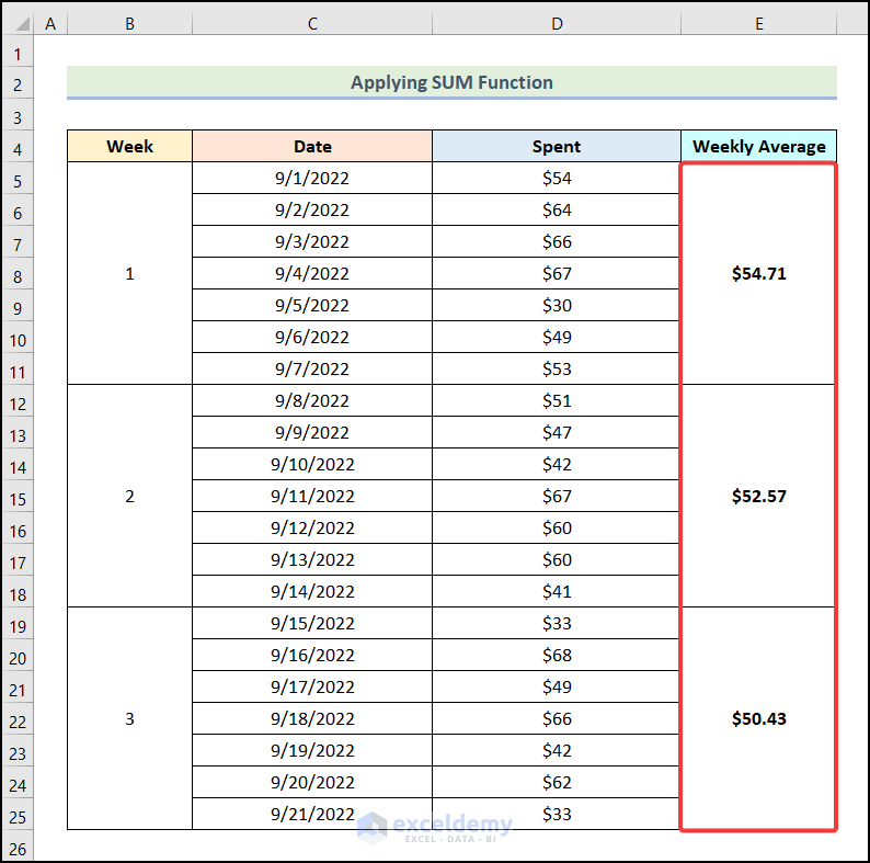
1.1 Applying the SUM Function to Calculate Weekly Average
Steps:
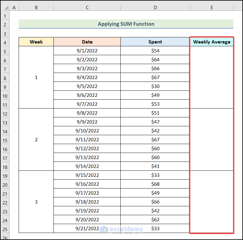
- Create a new Weekly Average column, as shown in the following image.
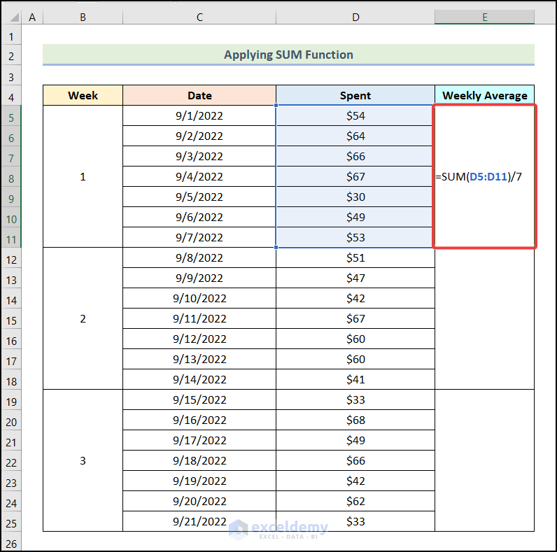
- Enter the formula given below in cell E5:
=SUM(D5:D11)/7The range D5:D11 refers to the first 7 cells of the Spent column.
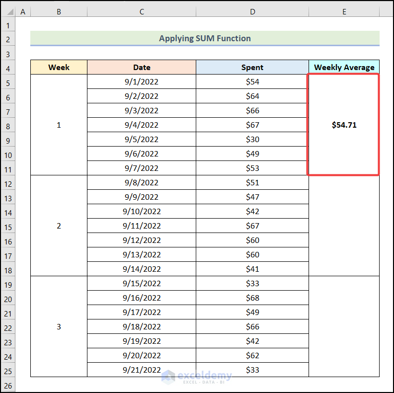
- Press ENTER.
You will have the weekly average for the 1st week, as marked in the following picture.
- Use the AutoFill feature of Excel to obtain the remaining outputs.
Read More: How to Calculate Daily Average in Excel
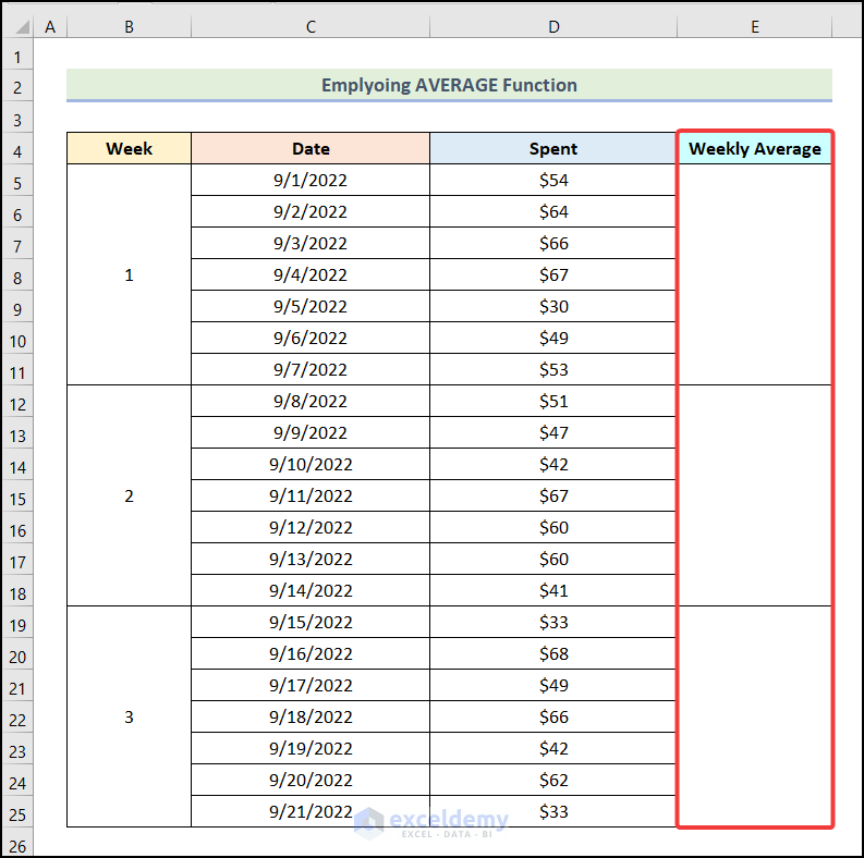
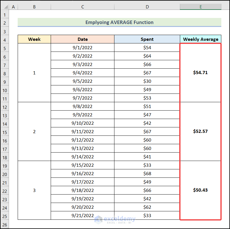
1.2 Applying the AVERAGE Function
Steps:
- Create a new column named Weekly Average, as shown in the image below.
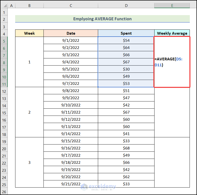
- Enter the following formula in cell E5:
=AVERAGE(D5:D11)The AVERAGE function will return the average value of the range D5:D11.
- Press ENTER.
You will have the weekly average for the 1st week, as demonstrated in the following image.
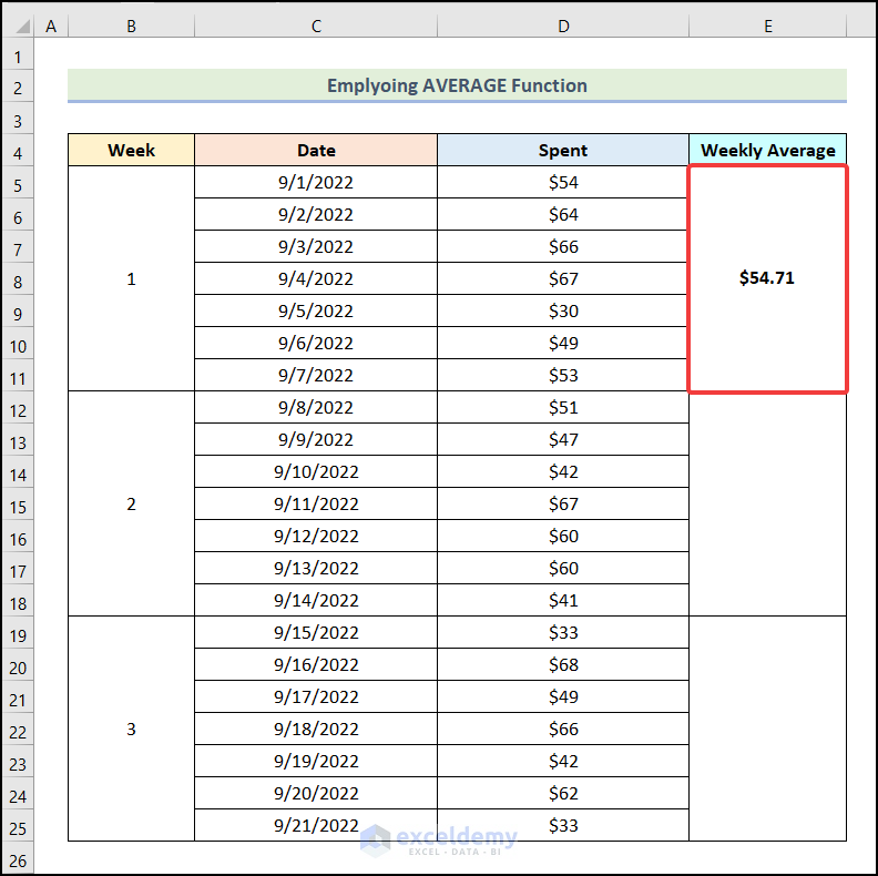
- Using the AutoFill option of Excel, you can have the rest of the outputs.
Read More: How to Calculate Monthly Average from Daily Data in Excel
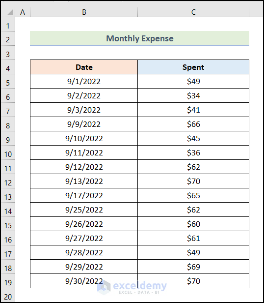
Method 2 – Computing Weekly Average from Monthly Data
We have Monthly Expenses as a dataset. We have the amount Spent for September. We aim to calculate the weekly average.
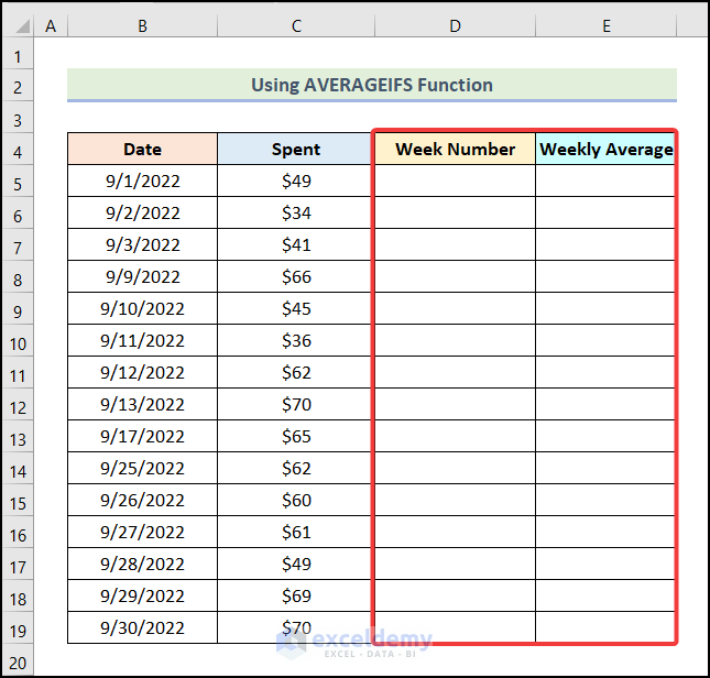
2.1 Using the AVERAGEIFS Function to Calculate Weekly Average
Steps:
- Create 2 new columns named Week Number and Weekly Average, as shown in the following image.
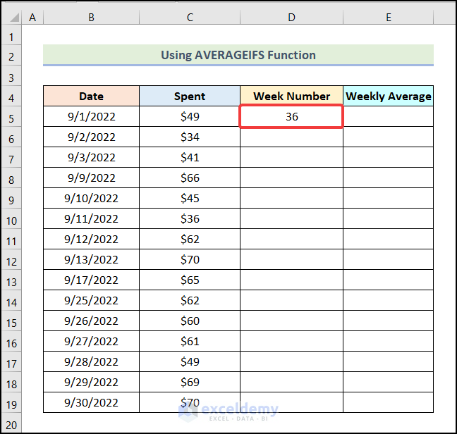
- Enter the following formula in cell D5:
=WEEKNUM(B5)Cell B5 represents the cell of the Date column. The WEEKNUM function will return the number of the week in the year for a specific date.
- Press ENTER.
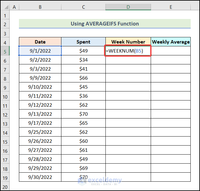
You will have the following output on your worksheet.
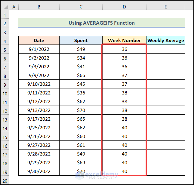
- Use the AutoFill option to get the rest of the Week Numbers, as shown in the following image.
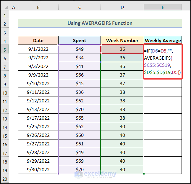
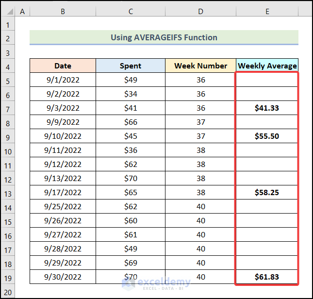
- Enter the following formula in cell E5:
=IF(D6=D5,"",AVERAGEIFS($C$5:$C$19,$D$5:$D$19,D5))Here, cell D6 refers to the 2nd cell of the Week Number column, cell D5 indicates the 1st cell of the Week Number column, the range $C$5:$C$19 represents the cells of the Spent column, and the range $D$5:$D$19 indicates the cells of the Week Number column.
Formula Breakdown
- AVERAGEIFS($C$5:$C$19,$D$5:$D$19,D5) → This returns the average of a selected range based on one or more criteria.
- $C$5:$C$19 → It is the average_range argument.
- $D$5:$D$19 → This refers to the criteria_range1 argument.
- D5 → It represents the criteria1 argument.
- Output → 41.33
- IF(D6=D5,””,AVERAGEIFS($C$5:$C$19,$D$5:$D$19,D5)) → It becomes IF(D6=D5,””,41.33).
- The IF function returns a value if the specified condition is met and returns another value if the specified condition is not met. In this case, if the next cell (D6) becomes equal to the current cell (D5), there are more entries of the current Week Number. So if this condition is satisfied, keep the cell blank (“”). But when the next cell is not equal to the current cell that means the Week Number has changed. So, we will show the value from the AVERAGEIFS function.
- D6=D5 → It is the logical_test argument.
- “” → This refers to the [value_if_true] argument.
- 41.33 → It is the [value_if_false] argument.
- Output → Blank cell.
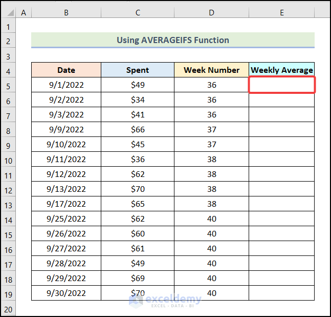
- Press ENTER.
You will see a blank output in cell E5 as it is not the last entry of the 36th week.
- Use the AutoFill option to get the Weekly Average of all the weeks, as shown in the image below.
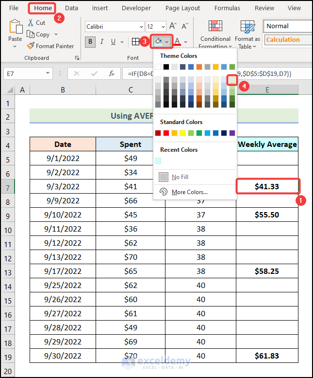
You can add a fill to the output cells to make them stand out. To do this, let’s follow the steps given below.
- Go to the Home tab from Ribbon.
- Select the Fill Color option from the Font group.
- Choose your preferred color from the drop-down.
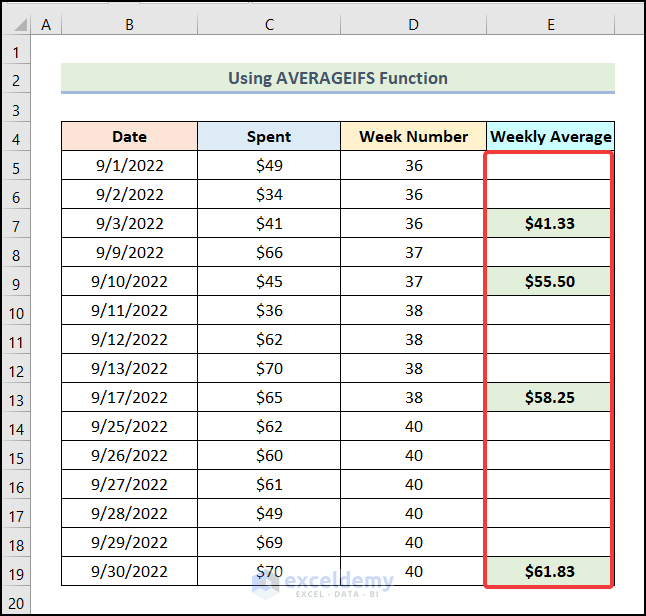
- Follow the same steps to apply the Fill Color in the remaining outputs.
Your final output table will look like the following picture.
Read More: How to Calculate Average of Multiple Columns in Excel
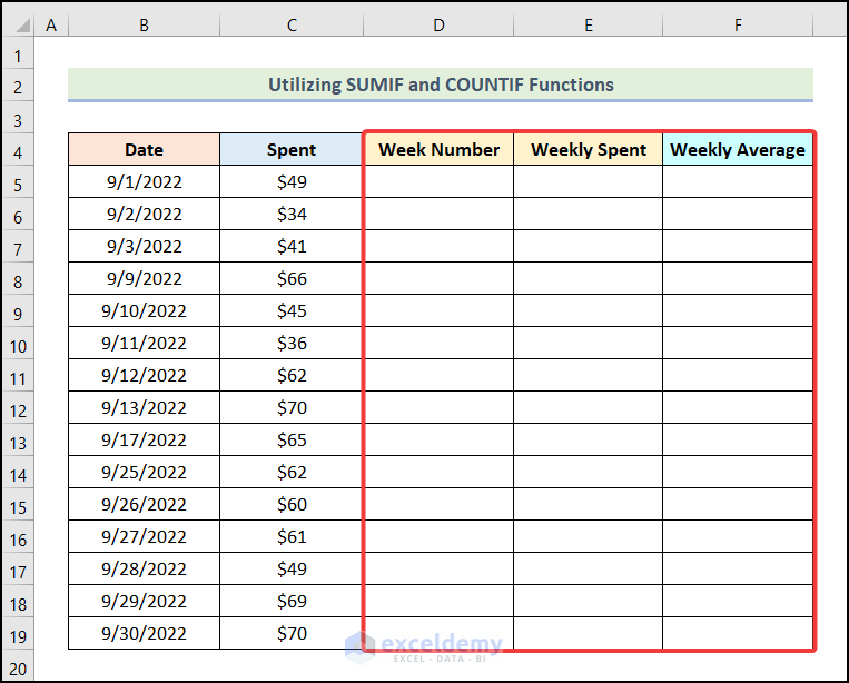
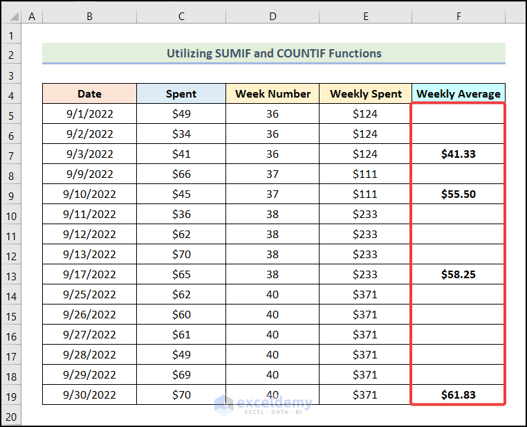
2.2 Utilizing SUMIF and COUNTIF Functions
Steps:
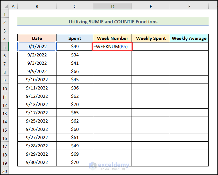
- Create 3 new columns named Week Number, Weekly Spent, and Weekly Average.
- Enter the following formula in cell D5:
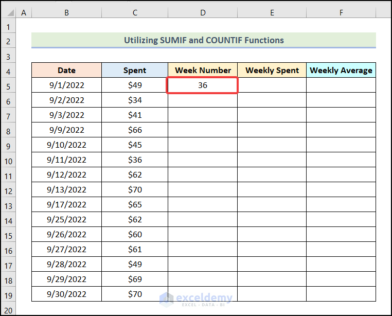
=WEEKNUM(B5)- Press ENTER.
You will have the Week Number for the Date in cell B5.
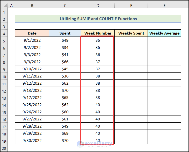
- Using the AutoFill feature, get the rest of the outputs, as shown in the image below.
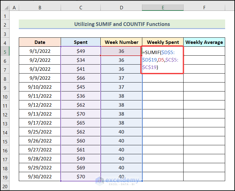
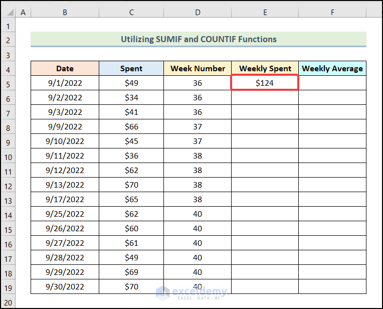
- Enter the following formula in cell E5:
=SUMIF($D$5:$D$19,D5,$C$5:$C$19)Here, the cell D5 indicates the 1st cell of the Week Number column, the range $D$5:$D$19 refers to the cells of the Week Number column, and the range $C$5:$C$19 represents the cells of the Spent column.
Now, the SUMIF function will return the sum of the cells in the range $C$5:$C$19 based on the Week Number.
- Press ENTER.
You will have the Weekly Spent amount for Week Number 36 in cell E5.
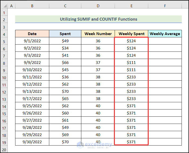
- Use the AutoFill feature to get the Weekly Spent amount for all Week Numbers.
- Enter the following formula in cell F5:
=IF(D6=D5,"",E5/COUNTIF($D$5:$D$19,D5))Here, cell D6 refers to the 2nd cell of the Week Number column, and cell E5 represents the 1st cell of the Weekly Spent column.
Formula Breakdown
- COUNTIF($D$5:$D$19,D5) → This counts the cells in the range $D$5:$D$19 based on the Week Number.
- $D$5:$D$19 → It is the range argument.
- D5 → This refers to the criteria argument.
- Output → 3.
- IF(D6=D5,””,E5/COUNTIF($D$5:$D$19,D5)) → It becomes IF(D6=D5,””,E5/3).
- D6=D5 → It is the logical_test argument.
- “” → It represents the [value_if_true] argument.
- E5/3 → This refers to the [value_if_false] argument.
- Output → Blank cell.
- Press ENTER.
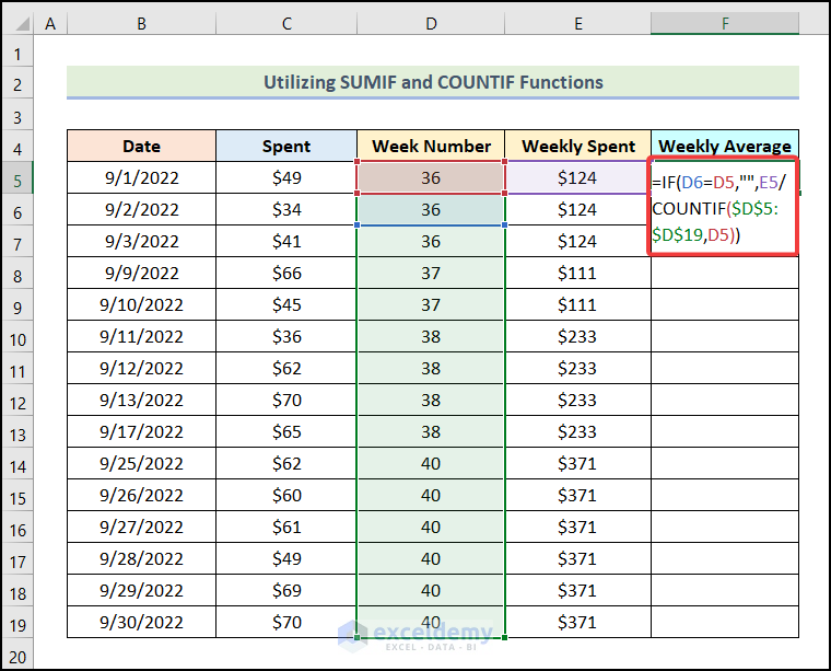
You will have a blank cell as output in cell F5, as it is not the last entry of the 36th week.
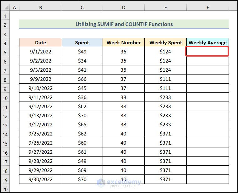
- Use the AutoFill feature to get the weekly average for each week, as demonstrated in the following picture.
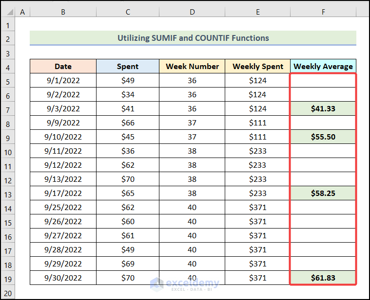
- Following the steps from the previous method, apply Fill Color to the output cells.
Your final output table will look like the following image.
Read More: How to Get Average Time in Excel
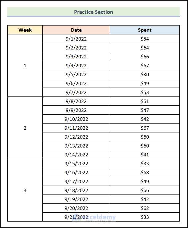
Practice Section
We have provided a Practice Section on the right side of the Excel Workbook.
Download the Practice Workbook
Related articles
- How to Calculate Average Rating in Excel
- How to Calculate 5 Star Rating Average in Excel
- How to Calculate Average Growth Rate in Excel
- How to Calculate Daily Average from Hourly Data in Excel
<< Go Back to How to Calculate Average in Excel | How to Calculate in Excel | Learn Excel
Get FREE Advanced Excel Exercises with Solutions!
