Method 1 – Calculate Monthly Average from Daily Data with SUM Function in Excel
STEPS:
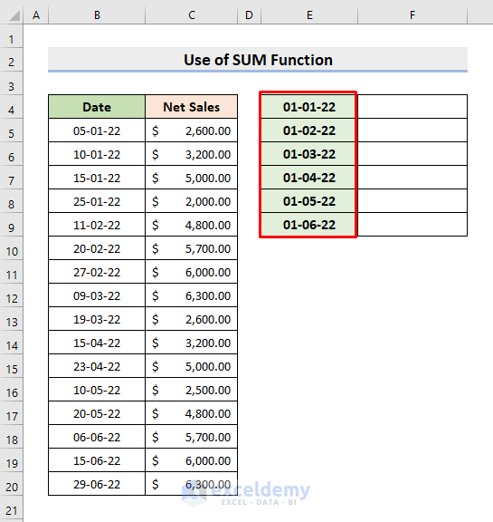
- Input the name of the month first.
- Select the range E4:E9.
- Type the first day of each month respectively in each cell.
- See the picture below to understand better.
- Select the range again and press the Ctrl and 1 keys together.
- The Format Cells dialog box will pop out.
- Under the Number tab, choose Category > Custom and Type > mmmm.
- Press OK.
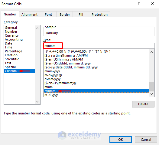
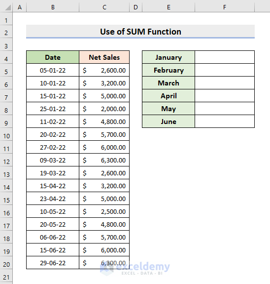
- It’ll return the accurate name of the months.
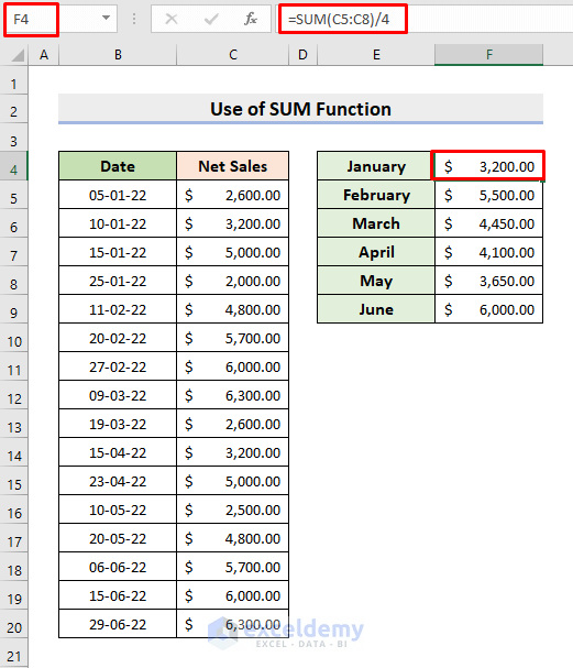
- Select cell F4.
- Type the formula:
=SUM(C5:C8)/4- Press Enter.
- You’ll get the average net sales for January.
- We divide it by 4 as January month has 4 inputs.
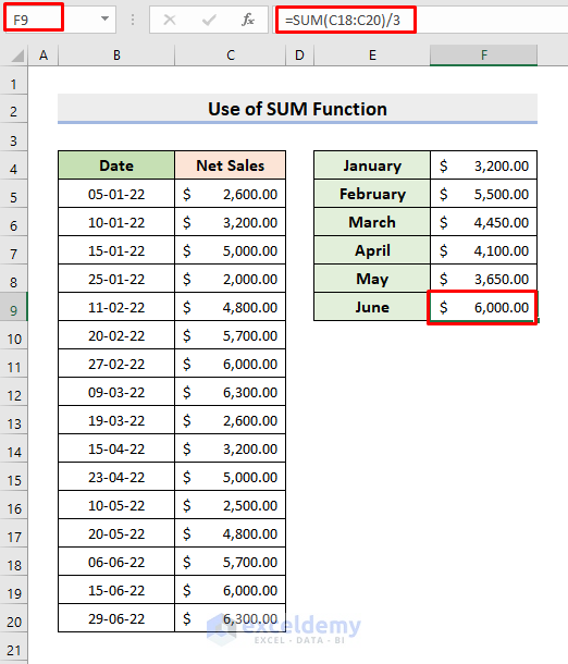
- Apply AutoFill as the data inputs don’t maintain a pattern.
- Type the formulas manually.
- See the formula in F9 for June is:
=SUM(C18:C20)/3- Get the monthly average from daily data.
Method 2 – Insert AVERAGE Function for Computing Daily Data Average by Month
STEPS:
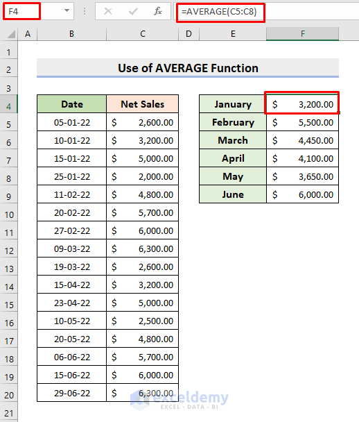
- Choose cell F4.
- Input the formula:
=AVERAGE(C5:C8)- Click Enter.
- It’ll return the average of January.
- Use AutoFill here.
- Select the average range by checking the date inputs per month.
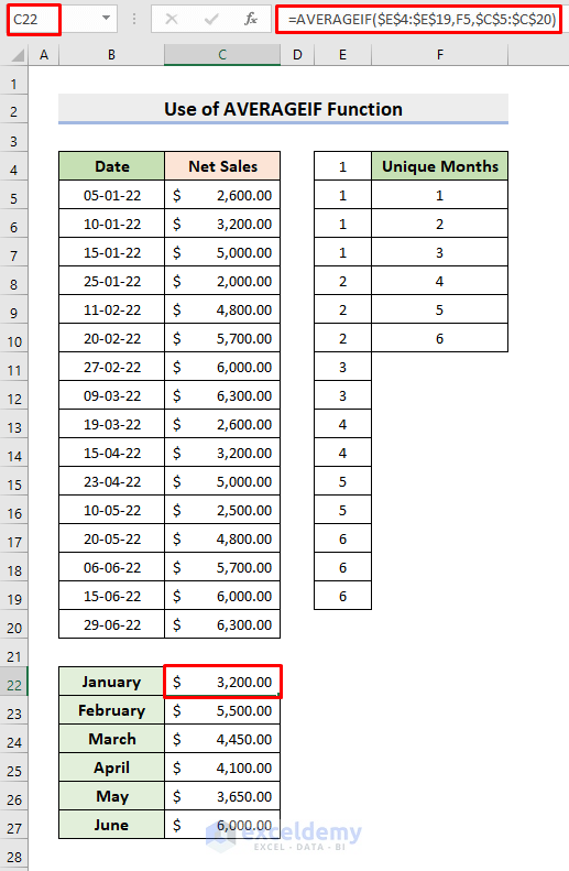
Method 3 – Use AVERAGEIF Function to Determine Monthly Average in Excel.
STEPS:
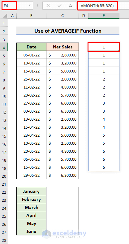
- Click cell E4.
- Insert the formula:
=MONTH(B5:B20)- Hit Enter.
- Spill the monthly numbers.
- Look at the figure below.
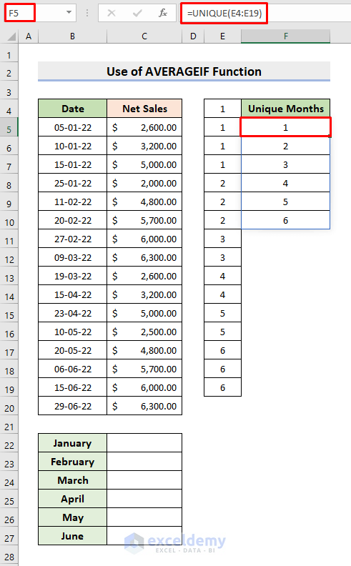
- You will need the unique month numbers instead of a single month appearing multiple times.
- The UNIQUE function gives out distinct cell values from a range.
- Select cell F5.
- Type the formula:
=UNIQUE(E4:E19)- Spill the distinct month numbers.
- Choose cell C22.
- Input the formula:
=AVERAGEIF($E$4:$E$19,F5,$C$5:$C$20)- $E$4:$E$19 is the criteria range, F5 is the desired condition, and $C$5:$C$20 is the sales range from where we’ll find the average.
- Press Enter.
- Use AutoFill to get other outputs.
- Obtain the monthly average values from daily data.
Method 4 – Get Daily Data Average by Month Through AVERAGEIFS Function
STEPS:
- Select cell F4.
- Type the formula:
=AVERAGEIFS($C$5:$C$20,$B$5:$B$20,">="&E4,$B$5:$B$20,"<="&EOMONTH(E4,0))- Press Enter.
- Apply AutoFill.
- Get the monthly average values.
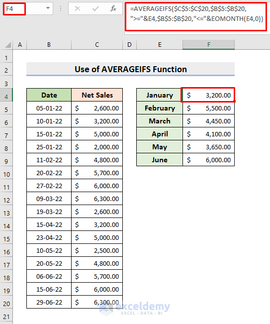
NOTE: $C$5:$C$20 is the average range. The condition range is $B$5:$B$20 for both cases. “>=”&E4 is the first condition. It looks for values that are greater than the first day of January. The second condition is “<=”&EOMONTH(E4,0), which looks for data lower than the last day of January.
Method 5 – Apply Excel Pivot Table to Calculate Monthly Average
STEPS:
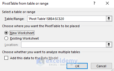
- Select the range B4:C20.
- Go to Insert > PivotTable.

- A dialog box will appear.
- Press OK.
- Drag the Date and the Months fields and drop them under the Rows section.
- Drag the Net Sales field and place it under the Values.
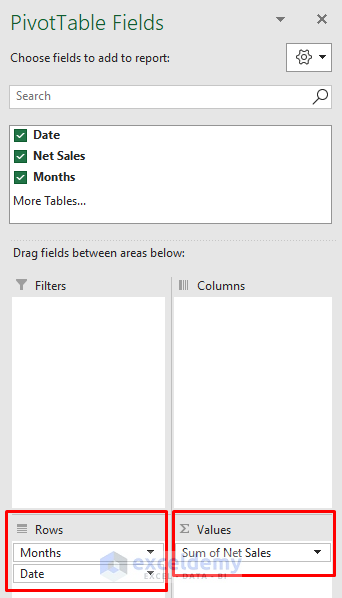
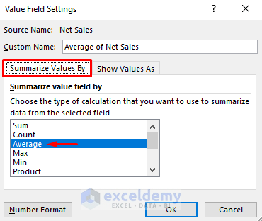
- Choose Value Field settings from the Sum of Net Sales drop-down.
- The dialog box will emerge.
- Click Average from the Summarize Values By options.
- Hit OK.
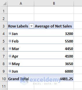
- A new worksheet will appear containing the monthly average net sales.
Download Practice Workbook
Download the following workbook to practice by yourself.
Related Articles
- How to Calculate Average Rating in Excel
- How to Calculate 5 Star Rating Average in Excel
- How to Calculate Average Growth Rate in Excel
- How to Get Average Time in Excel
<< Go Back to How to Calculate Average in Excel | How to Calculate in Excel | Learn Excel
Get FREE Advanced Excel Exercises with Solutions!
