Method 1 – Calculate a 5 Star Rating Average Using SUM Function
STEPS:
- In cell E5, enter the following formula:
=C5*D5
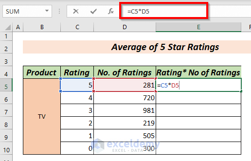
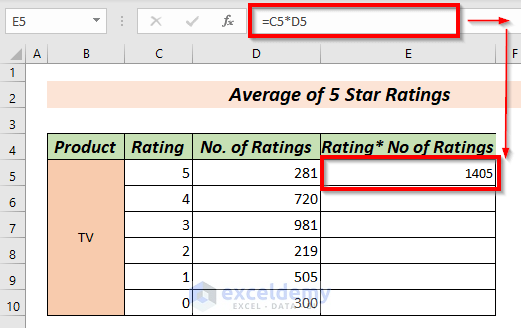
- Press ENTER to get the value of the product of Rating and No of Ratings in the Rating * No of Ratings column.
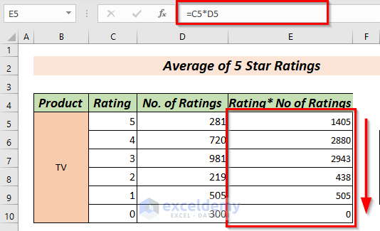
- By dragging down the Fill Handle, we can use Excel’s AutoFill feature to get values in other cells in the Rating * No of Ratings column.
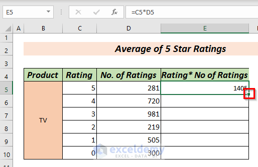
- We will get corresponding values in other cells as well.
- Get the sum of Rating * No of Ratings column and divide it by the sum of No of Ratings column.
- To do so,
- Use the SUM Function of Excel.
- In cell G8, enter the following formula:
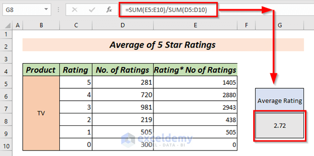
=SUM(E5:E10)/SUM(D5:D10)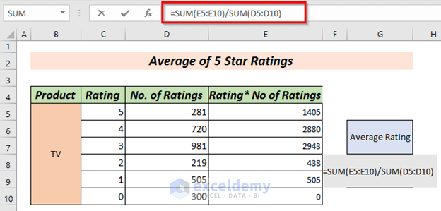
Formula Breakdown
SUM(E5:E10) >> Shows us the sum of E5 to E10 cells in the Rating * No of Ratings column.
Output is >> 8171
SUM(D5:D10)>> Shows us the sum of E5 to E10 cells in the Rating column.
Output is>>3006
SUM(E5:E10)/SUM(D5:D10)>> Shows us the result of dividing the first sum by the latter.
Output is>> 8171/3006 =2.72
Explanation: Here, it shows the average of 5-star ratings.
- Press ENTER to get an average of 5-star ratings.
Read More: How to Calculate Average Rating in Excel
Method 2 – Calculate a 5 Star Rating Average Using the SUMPRODUCT Function
STEPS:
- In cell G8, enter the following formula:
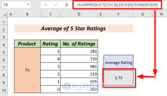
=SUMPRODUCT(C5:C10,D5:D10)/SUM(D5:D10)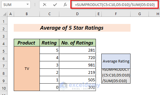
Formula Breakdown
SUMPRODUCT(C5:C10,D5:D10)>> First, the SUMPRODUCT Function will multiply the Rating column by the No. of Ratings column. Then, it will sum all the results of multiplication.
Output is >> 8171
SUM(D5:D10)>> Shows us the sum of E5 to E10 cells in the Rating column.
Output is>>3006
SUMPRODUCT(C5:C10,D5:D10)/SUM(D5:D10)>> This shows us the result of dividing the first sum by the latter.
Output is>>8171/3006 = 2.72
Explanation: Here, it shows the average of 5-star ratings.
- Press ENTER to get an average of 5-star ratings.
Read More: How to Calculate Sum & Average with Excel Formula
Method 3 – Using SUM and COUNT Functions
STEPS:
- Enter the following formula in cell F8:
=SUM(D5:D12)/COUNT(C5:C12)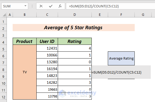
Formula Breakdown
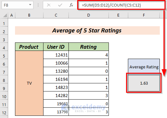
SUM(D5:D12)>> First, the SUM Function will sum all the cells in the Rating column.
Output is >> 13
COUNT(C5:C12)>> Shows us the number of cells with values in the User ID column.
Output is>>8
SUM(D5:D12)/COUNT(C5:C12)>> Shows us the result of dividing the first sum by the number of cells in the User ID column.
Output is>>13/8 =1.63
Explanation: Here, it shows the average of 5-star ratings.
- Press ENTER to get an average of 5-star ratings.
Things to Remember
SUMPRODUCT Function does the job of sum and product in a single function. You can avoid first getting the product of the numbers and then getting the sum by using this function. It will enable you to skip a step and save time.
Practice Section
We have included a practice section so you can practice the methods.
Download the Practice Workbook
Related Articles
- How to Calculate Average Growth Rate in Excel
- How to Get Average Time in Excel
- How to Calculate Daily Average in Excel
- How to Calculate Daily Average from Hourly Data in Excel
- How to Calculate Weekly Average in Excel
- How to Calculate Monthly Average from Daily Data in Excel
<< Go Back to Excel Average Formula Examples | How to Calculate Average in Excel | How to Calculate in Excel | Learn Excel
Get FREE Advanced Excel Exercises with Solutions!
