Method-1 – Using AVERAGE, ROWS, and OFFSET Functions to Calculate Daily Average from Hourly Data in Excel
We will calculate the daily averages for views from 9/20/2022 to 9/24/2022 using the AVERAGE, OFFSET, and ROWS functions.
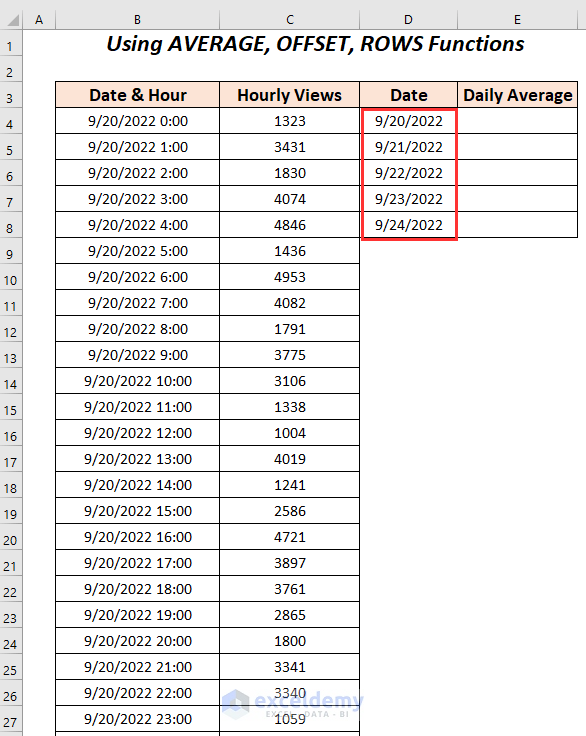
Steps:
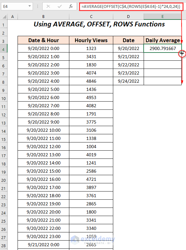
- Type the following formula in cell E4.
=AVERAGE(OFFSET(C$4,(ROWS(E$4:E4)-1)*24,0,24))Formula Breakdown
- ROWS(E$4:E4) → returns the number of range of rows from E$4:E4.
- Output → 1
- ROWS(E$4:E4)-1 → becomes
- 1-1 → 0
- (ROWS(E$4:E4)-1)*24 → becomes
- 0*24 → 0
- OFFSET(C$4,(ROWS(E$4:E4)-1)*24,0,24) → becomes
- OFFSET(C$4,0,0,24) → extracts a range from C$4 with a height of 24
- Output → $C$4:$C$27
- OFFSET(C$4,0,0,24) → extracts a range from C$4 with a height of 24
- AVERAGE(OFFSET(C$4,(ROWS(E$4:E4)-1)*24,0,24)) → becomes
- AVERAGE($C$4:$C$27) → returns the average value of the views of the range $C$4:$C$27 for 24 hours of 9/20/2022.
- Output → 2900.791667
- AVERAGE($C$4:$C$27) → returns the average value of the views of the range $C$4:$C$27 for 24 hours of 9/20/2022.
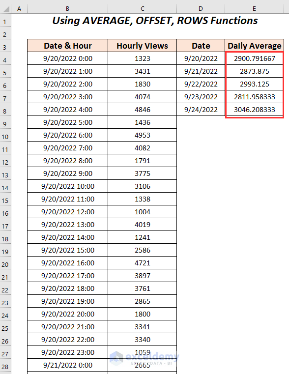
- Press ENTER and drag down the Fill Handle.
Get the daily averages of hourly views from 9/20/2022 to 9/24/2022.
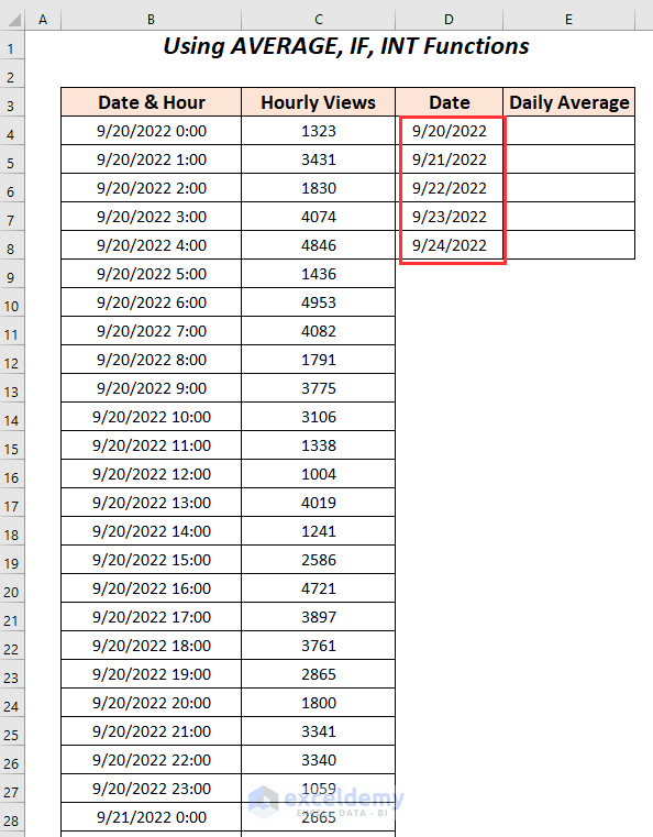
Method-2 – Using AVERAGE, IF, & INT Functions to Calculate Daily Average from Hourly Data in Excel
We will use the AVERAGE, IF, and INT functions to calculate the daily averages for views from 9/20/2022 to 9/24/2022.
Steps:
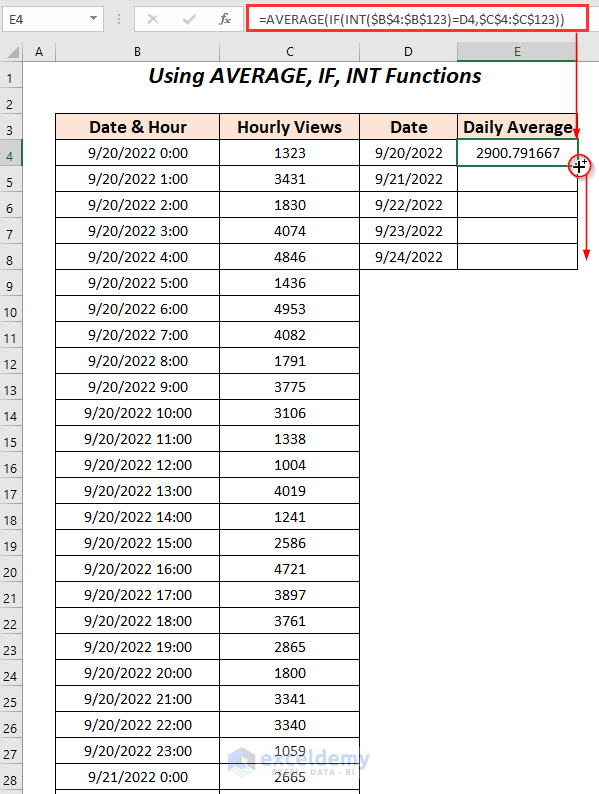
- Apply the following formula in cell E4.
=AVERAGE(IF(INT($B$4:$B$123)=D4,$C$4:$C$123))The INT function will return the integer values of the range $B$4:$B$123 by extracting only date values. The IF function will check if the values match the date 9/20/2022. For matching values, TRUE will appear, and for other non-matched values, FALSE will appear. Those hourly values will be returned among the range $C$4:$C$123, for which we have TRUE for the corresponding rows.
The AVERAGE function will return the average value.
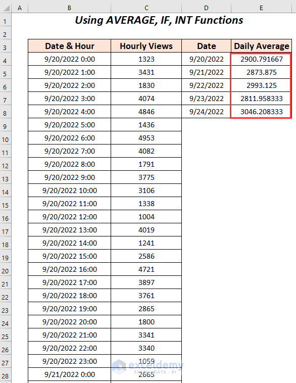
- Press ENTER and drag down the Fill Handle.
Get the daily averages of hourly views from 9/20/2022 to 9/24/2022.
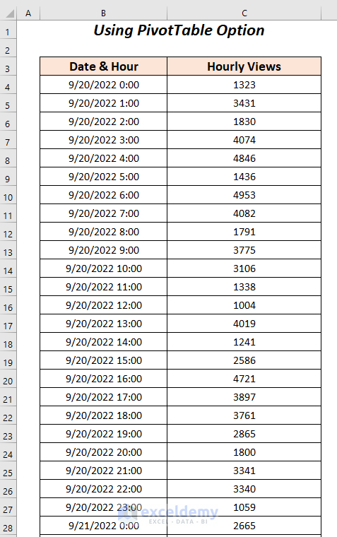
Method-3 – Implementing PivotTable to Calculate Daily Average from Hourly Data in Excel
Utilize the PivotTable option for daily average hourly views from 9/20/2022 to 9/24/2022.
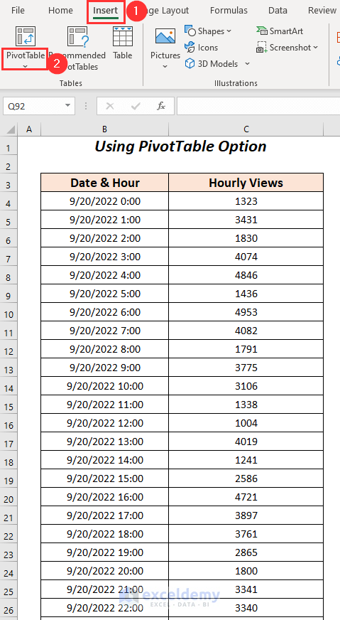
- Go to the Insert tab >> PivotTable.
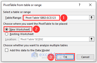
The PivotTable from the table or range dialog box will open up.
- Select the range as Table/Range.
- Click on the New Worksheet option and press OK.
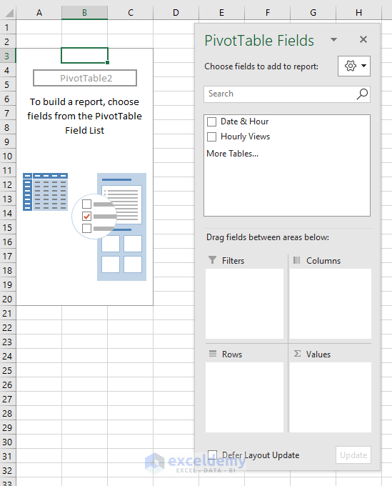
You will be taken to a new sheet with two portions: a PivotTable on the left side and PivotTable Fields on the right side.
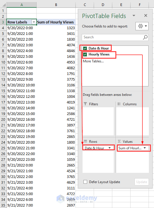
- Drag down the Date & Hour field to the Rows area and the Hourly Views field to the Values.
In the Values area, click on the dropdown symbol next to the field Sum of Hourly Views to select the Value Field Settings option.
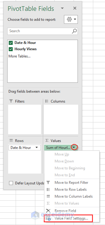
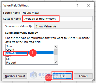
The Value Field Settings wizard will open up.
- Select the Average option and press OK.
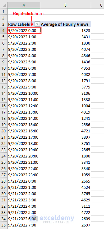
The Custom Name will be changed to Average of Hourly Views.
- Right-click on any cell of the Row Labels indicated column.
- Choose the Group option among various options.
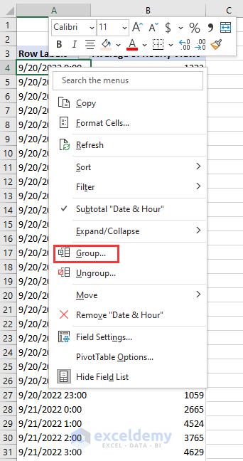
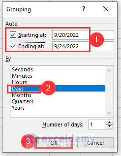
The Grouping dialog box will appear.
- Check the boxes Starting at with the date 9/20/2022 and Ending at with the date 9/24/2022 and select the Days
- Press OK.
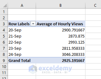
You will get the average hourly views for each day.
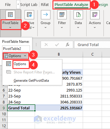
- To stop seeing the total amount, go to the PivotTable Analyze tab >> PivotTable group >> Options dropdown >> Options.
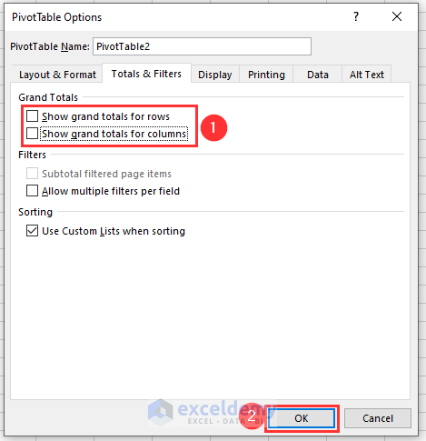
The PivotTable Options wizard will appear.
- In the Total & Filters tab, uncheck the Show grand totals for rows and Show grand totals for columns
- Press OK.
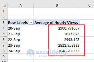
Get the following table with our average views per day.
Download Workbook
Related Articles
- How to Calculate Average Rating in Excel
- How to Calculate 5 Star Rating Average in Excel
- How to Calculate Average Growth Rate in Excel
- How to Get Average Time in Excel
- How to Calculate Weekly Average in Excel
<< Go Back to How to Calculate Average in Excel | How to Calculate in Excel | Learn Excel
Get FREE Advanced Excel Exercises with Solutions!
