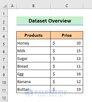
For illustration, the sample dataset below will be used to calculate average, minimum, and maximum in Excel.
Method 1: Use Functions to Calculate Average, Minimum And Maximum in Excel
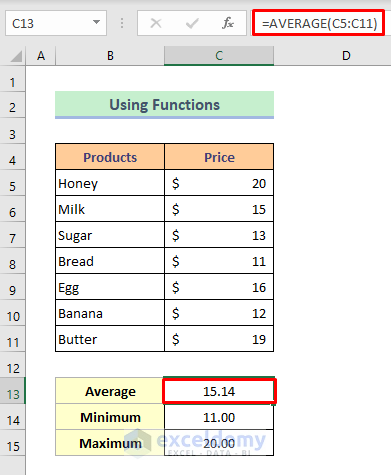
The AVERAGE function calculates the average (arithmetic mean) of a group of numbers.
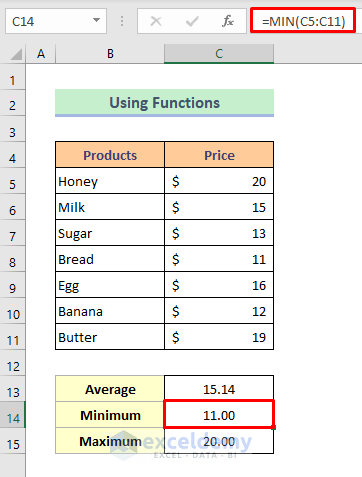
The MIN function returns the smallest value.
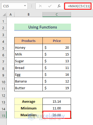
The MAX function returns the highest value.
Step 1:
➦ In Cell C13 enter the formula below
=AVERAGE(C3:C9)➦ Hit ENTER to get the average.
Step 2:
➦ Activate Cell C14 and enter the formula
=MIN(C3:C9)➦ Hit ENTER to get the minimum value.
Step 3:
➦ Enter the formula below in Cell C15
=MAX(C3:C9)➦ Hit ENTER to find the maximum value.
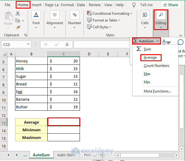
Method 2: Applying AutoSum Tool
Step 1:
➦ Activate Cell C13.
➦ Click Home > Editing > AutoSum > Average.
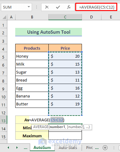
Step 2:
➦ Select the data range and hit Enter.
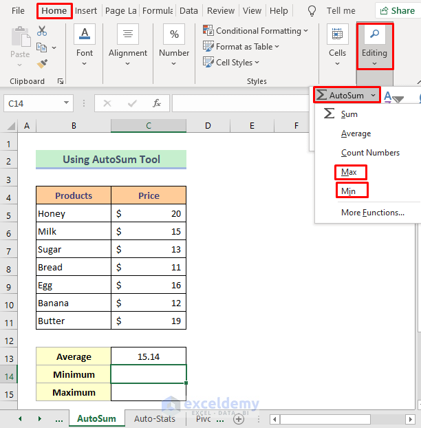
➦ Click HOME > Editing > AutoSum > Min/Max. Follow the other steps mentioned in the previous method.
Read More: How to Average Values Greater Than Zero in Excel
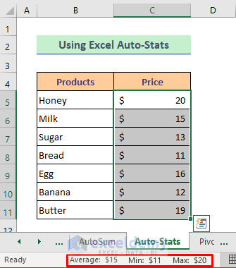
Method 3: Utilizing Auto-Stats Feature
➦ Select the data range and Excel will automatically show the Average, Min, and Max values in the status bar of your sheet.
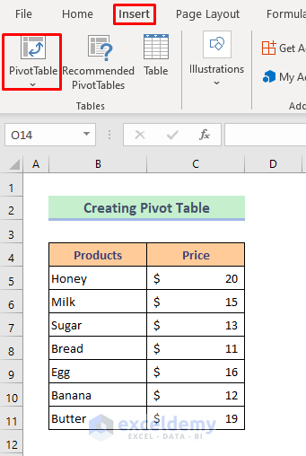
Method 4: Create Pivot Table to Calculate Average Minimum And Maximum
Step 1:
➦ Click Insert > PivotTable.
➦ A dialog box will open up.
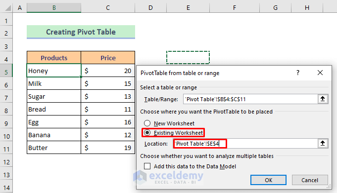
Step 2:
➦ Select where you will create the table and set the location. I have selected Existing Worksheet and Cell E4 as the location.
➦ Press OK.
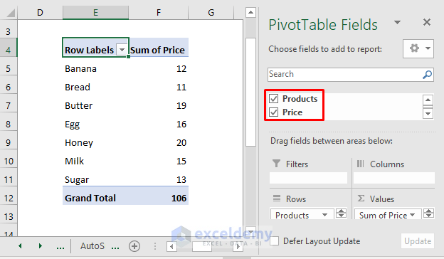
➦ A dialog box named ‘PivotTable Fields’ will appear.
Step 3:
➦ Checkmark the Products and Price option in the field.
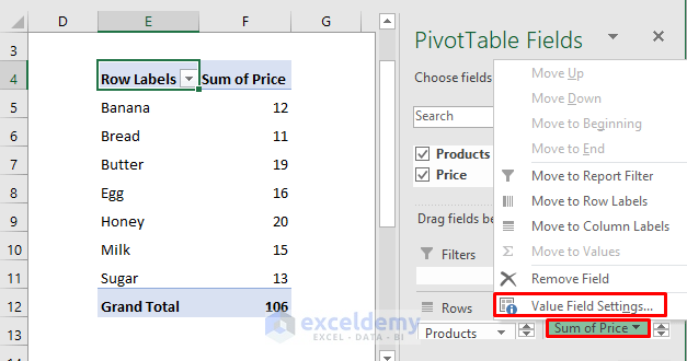
Step 4:
➦ Click Sum of Price > Value Field Settings.
➦ Value Field Settings dialog box will appear.
Step 5:
➦ Select Average from the ‘Summarize Values By’ option and press OK.
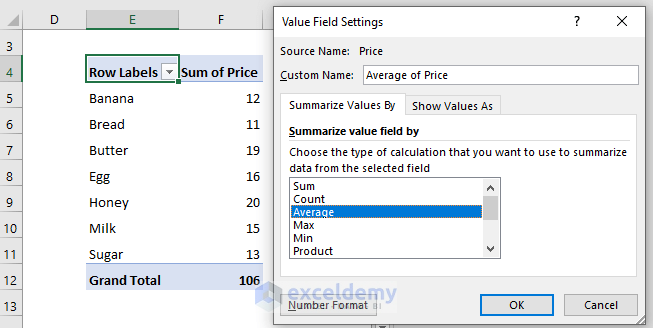
Excel will show the average price.
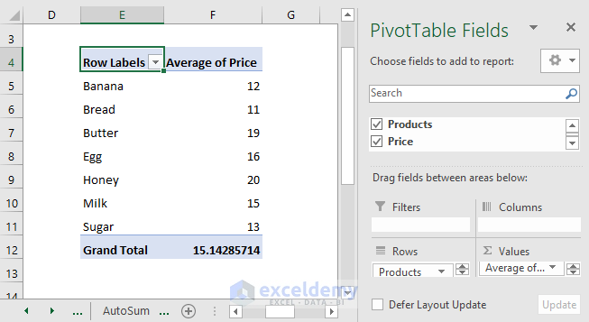
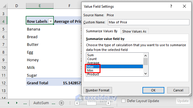
Step 6:
➦ To find the minimum or maximum, select Max/Min from the ‘Summarize Values By’ option and press OK.
Read More: How to Average Negative and Positive Numbers in Excel
How to Find Average, Minimum and Maximum Value with Condition in Excel
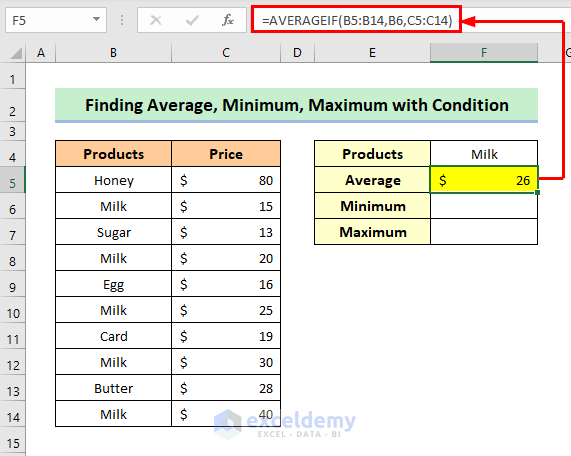
Let’s say, we want to calculate the average, minimum and maximum price of “Milk”.
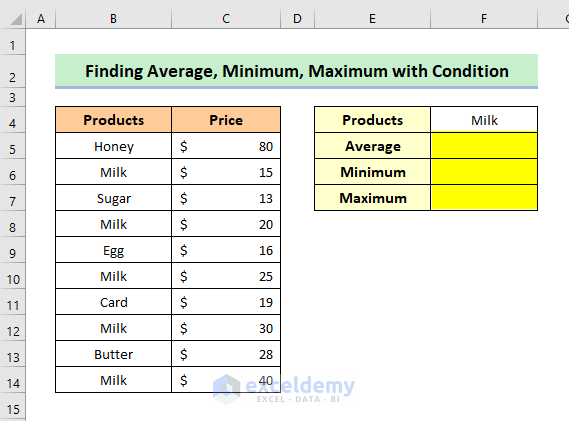
Step 1:
➦ In Cell F5 enter the formula given below
=AVERAGEIF(B5:B14,B6,C5:C14)
➦ Press ENTER and the average will be calculated.
Step 2:
➦ Activate Cell C14 and enter the formula
=MIN(IF(B5:B14=F4,C5:C14))
➦ Press ENTER to get the minimum value.
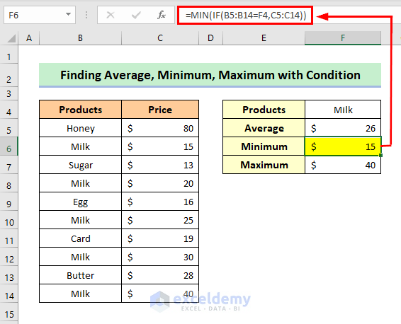
💡 Formula Breakdown
The IF function looks for the cell value of F4 in the range, B5:B14 returns the corresponding value of F4 from the range C5:C14.
Output => {FALSE;15;FALSE;20;FALSE;25;FALSE;30;FALSE;40}
The MIN function returns the minimum value from the array.
MIN(IF(B5:B14=F4,C5:C14)) = MIN({FALSE;15;FALSE;20;FALSE;25;FALSE;30;FALSE;40}) = 15
Final Output => 15
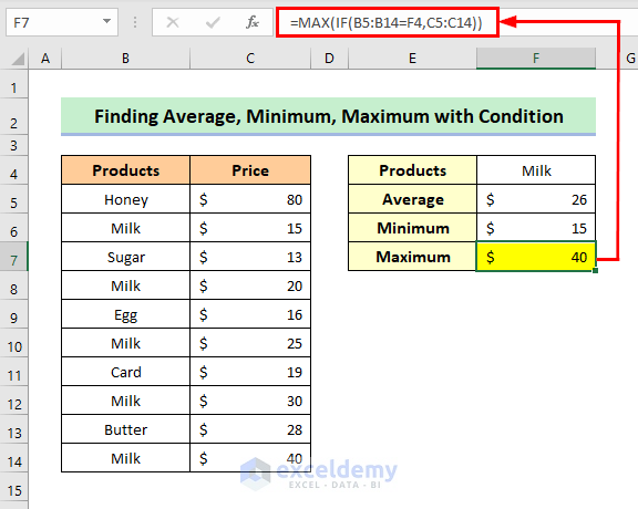
Step 3:
➦ Enter the formula in Cell C15
=MAX(IF(B5:B14=F4,C5:C14))
➦ Press ENTER to find the maximum value.
Read More: How to Average Filtered Data in Excel
Download Practice Book
Related Articles
- Average Attendance Formula in Excel
- How to Calculate Average of Averages in Excel
- How to Calculate Average True Range in Excel
- How to Calculate Average Percentage in Excel
- How to Calculate Average Percentage of Marks in Excel
- How to Calculate Class Average in Excel
- How to Calculate Average Revenue in Excel
- How to Calculate Average Quarterly Revenue in Excel
- How to Calculate Average Share Price in Excel
- How to Calculate Average Length of Stay in Excel
- How to Calculate Average Price in Excel
<< Go Back to Calculate Average in Excel | How to Calculate in Excel | Learn Excel
Get FREE Advanced Excel Exercises with Solutions!

I’m confused. I download the excel file and send a copy to my drive.
Maybe anyday you delete this excel file which you share here & i download it then send my drive & save in excel when you delete this file can i there’s a chance to lost my saved this file
Hello Mahedi, thanks for your feedback. When you download the file then there’s no connection between your downloaded file and our uploaded file. So, no worries, your file won’t lose.