The average of a range of data doesn’t always illustrate the perfect pictures. Sometimes there are outliers in the range that cause a deviation from true averages, means, modes, or any other statistics. Occasionally, these deviations can be very drastic. So we need to find the desired values excluding outliers’ values sometimes to get a clear picture. In this article, we will see how to calculate the average excluding outliers in Excel.
What Is Outlier?
In statistics, an outlier is a data point that differs from the rest of the data points significantly. In other words, outliers are inconsistencies among statistical distributions. Usually, these values are significantly larger or smaller than the rest of the values. When we combine these outliers with general values, the general idea for a group can often be misunderstood. So, it is very important to identify and remove outliers from some calculations.
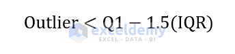
Statistically, an outlier abides by two conditions. For outliers that are significantly smaller than the rest, the condition is:
For larger values, the condition for the outliers is:
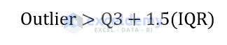
Where Q1, Q3, and IQR are 1st quartile, 3rd quartile, and interquartile range respectively.
How to Calculate Average Excluding Outliers in Excel: 4 Easy Methods
We can use different functions, or combinations of functions to either ignore outliers while calculating averages or eliminate outliers altogether and then calculate the average or other calculations in Excel. Below is a demonstration of 4 methods that can help us to calculate the average excluding outliers in Excel. For every method, we are going to use the following dataset to calculate the average.
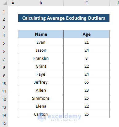
Here, we can see that there are two outliers in this dataset. In every method, we are going to calculate the average age of all people here ignoring these outliers.
1. Using TRIMMEAN Function
The TRIMMEAN function in Excel returns the average of a range of data excluding a top or bottom percentage of the values. It takes the array and the percentage to be ignored as the arguments. Follow these steps to see how you can use this function to calculate the average excluding outliers in Excel.
Steps:
- First, select a cell to enter the average (we have selected cell C16 here) and write down the following formula.
=TRIMMEAN(C5:C14,0.2)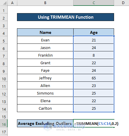
- Then press Enter on your keyboard. You will have the average excluding the outliers for this dataset.
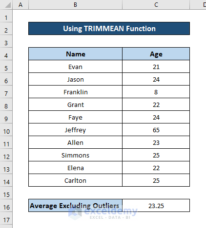
This function has taken the range C5:C14 as the array argument and ignored 20% of the values (2 out of 10 = 0.2 as the second argument) that included the top and bottom outliers combined. Then the function returned the average for the rest of the data.
Read More: How to Exclude a Cell in Excel AVERAGE Formula
2. Applying AVERAGEIFS Function
Excel has a function called the AVERAGEIFS function that can be used to calculate averages excluding outliers if done right. Unfortunately, if you use this function only to do the task, you have to manually input the outliers in the function.
This function takes the average range, different criteria ranges, and conditions as its arguments consecutively. It then returns the average of the range as its result. If we use the condition that eliminates the outliers with inequality conditions, we can easily calculate the average of a range excluding the outliers in Excel. Follow these steps for a more detailed guide.
Steps:
- First, select a cell to calculate the average and write down the following formula in it.
=AVERAGEIFS(C5:C14,C5:C14,">20",C5:C14,"<26")
- After pressing Enter you will finally have the average of the range in the dataset excluding the outliers.

🔍 Breakdown of the Formula
AVERAGEIFS(C5:C14,C5:C14,”>20″,C5:C14,”<26″)
👉 The AVERAGEIFS function calculates the mean of cell values that satisfy multiple criteria. Here, It considers only those values in the range C5:C14 that are greater than 20 and also less than 26. So, this formula calculates the mean of values in the range C5:C14 that fall between 20 to 26.
Read More: How to Calculate Average of Top 5 Values in Excel
3. Use of Interquartile Range
In the outliers section, we have seen the conditions of outliers with interquartile range. In statistics, an interquartile range is the distribution of the middle section of the dataset. We can easily calculate it by subtracting the 1st quartile from the 3rd in Excel. This can be done with the help of the QUARTILE function in Excel.
We can then use the OR function to determine which of the values are outliers in a range. This function takes different conditions as arguments and returns a boolean value depending on whether all the conditions are true or not. Then we can find the average for all the values eliminating the outliers with the help of the AVERAGEIFS function.
Follow these steps for an in-depth guide to the process.
Steps:
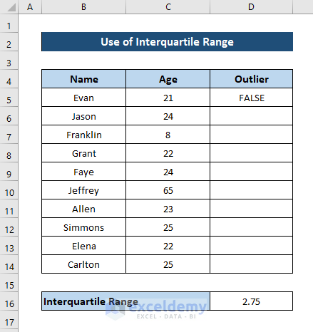
- First, select a cell for the interquartile range and write down the following formula in the cell.
=QUARTILE(C5:C14,3)-QUARTILE(C5:C14,1)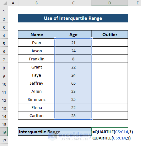
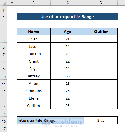
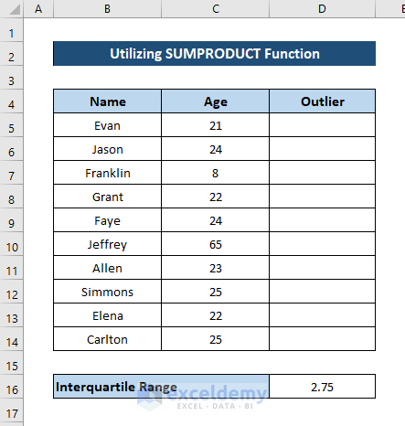
- Now press Enter and you will have the interquartile range of the dataset.
- After that, select cell D5 and write down the following formula.
=OR(C5<QUARTILE($C$5:$C$14,1)-1.5*$D$16,C5>QUARTILE($C$5:$C$14,1)+1.5*$D$16)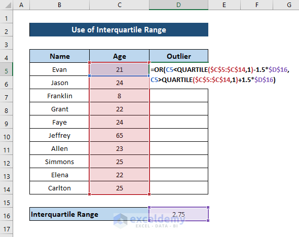
- Then press Enter and you will have a boolean value of whether the value of cell C2 is an outlier in the range or not.
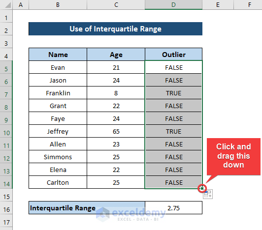
- Next, select the cell again and click and drag the fill handle icon to fill the rest of the cells of the column with the formula.
- After that, select a cell for the average and write down the following formula.
=AVERAGEIFS(C5:C14,D5:D14,FALSE)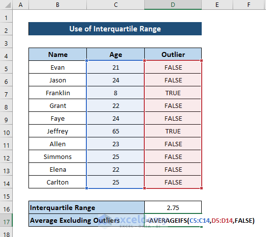
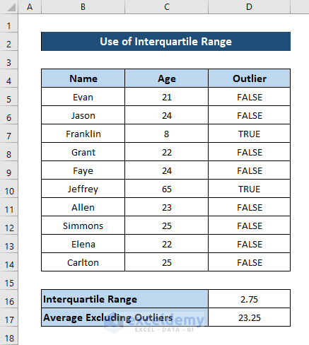
- Finally, press Enter. As a result, this will calculate the average of the dataset excluding outliers in Excel.
🔍 Breakdown of the Formula
OR(C5<QUARTILE($C$5:$C$14,1)-1.5*$D$16,C5>QUARTILE($C$5:$C$14,1)+1.5*$D$16)
👉 QUARTILE($C$5:$C$14,1) function takes the range C5:C14 as the array and returns the first quartile of this array.
👉 C5<QUARTILE($C$5:$C$14,1)-1.5*$D$16 is a condition that checks if the value of cell C5 is less than the difference between the first quartile of the range C3:C14 and 1.5 times of value in cell D16. Cell D16 here contains the interquartile range of the data.
👉 Whereas C5>QUARTILE($C$5:$C$14,1)+1.5*$D$16 condition checks if the value of cell C5 is greater than the sum of the third quartile of the range C5:C14 and 1.5 times the value of interquartile range which is at cell D16.
👉 Finally, OR(C5<QUARTILE($C$5:$C$14,1)-1.5*$D$16,C5>QUARTILE($C$5:$C$14,1)+1.5*$D$16) checks whether any of the two conditions described above is true or not. If either one is true, it returns the boolean value TRUE as output. Else, it returns FALSE.
4. Utilizing SUMPRODUCT Function
There is another function in Excel that can be utilized to calculate the average excluding outliers. It is called the SUMPRODUCT function. This function takes different ranges as arguments and returns the sum of the product of the corresponding range. We will also take the help of the QUARTILE function.
We can then use the OR function to determine which of the values are outliers in a range. This function takes different conditions as arguments and returns a boolean value depending on whether all the conditions are true or not.
Follow these steps to see how you can use the function to calculate the average excluding the outliers in Excel.
Steps:
- First, select a cell for the interquartile range and write down the following formula in the cell.
=QUARTILE(C5:C14,3)-QUARTILE(C5:C14,1)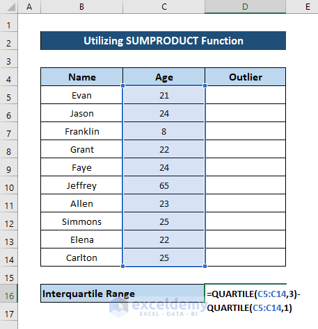
- Then press Enter and you will have the interquartile range of the dataset.
- After that, select cell D5 and write down the following formula.
=OR(C5<QUARTILE($C$5:$C$14,1)-1.5*$D$16,C5>QUARTILE($C$5:$C$14,1)+1.5*$D$16)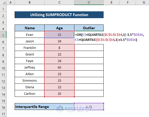
- Now press Ener and you will have a boolean value of whether the value of cell C2 is an outlier in the range or not.

- Next, select the cell again and click and drag the fill handle icon to fill the rest of the cells of the column with the formula.
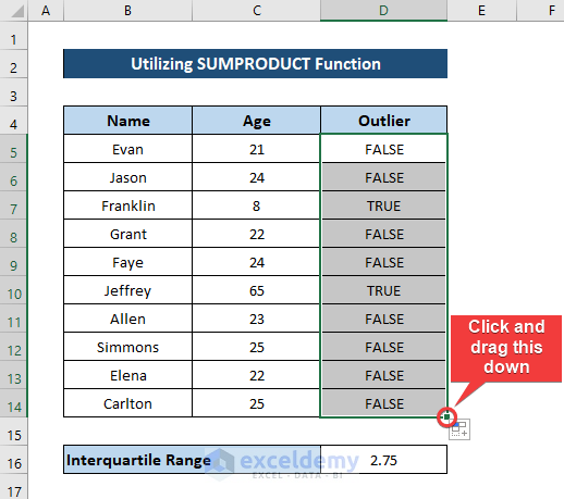
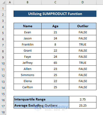
This will identify the outliers which are in cells D7 and D10.
🔍 Breakdown of the Formula
OR(C5<QUARTILE($C$5:$C$14,1)-1.5*$D$16,C5>QUARTILE($C$5:$C$14,1)+1.5*$D$16)
👉 QUARTILE($C$5:$C$14,1) function takes the range C5:C14 as the array and returns the first quartile of this array.
👉 C5<QUARTILE($C$5:$C$14,1)-1.5*$D$16 is a condition that checks if the value of cell C5 is less than the difference between the first quartile of the range C3:C14 and 1.5 times of value in cell D16. Cell D16 here contains the interquartile range of the data.
👉 Whereas C5>QUARTILE($C$5:$C$14,1)+1.5*$D$16 condition checks if the value of cell C5 is greater than the sum of the third quartile of the range C5:C14 and 1.5 times the value of interquartile range which is at cell D16.
👉 Finally, OR(C5<QUARTILE($C$5:$C$14,1)-1.5*$D$16,C5>QUARTILE($C$5:$C$14,1)+1.5*$D$16) checks whether any of the two conditions described above is true or not. If either one is true, it returns the boolean value TRUE as output. Else, it returns FALSE.
- Then select a cell for the average and write down the following formula in it.
=SUMPRODUCT((C5:C14>C7)*(C5:C14<C10)*(C5:C14))/SUMPRODUCT((C5:C14>C7)*(C5:C14<C10))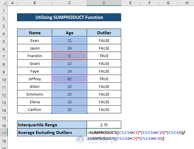
- Finally, press Enter and you will have the average of the dataset excluding outliers with the help of the SUMPRODUCT function in Excel.
🔍 Breakdown of the Formula
SUMPRODUCT((C5:C14>C7)*(C5:C14<C10)*(C5:C14))/SUMPRODUCT((C5:C14>C7)*(C5:C14<C10))
👉 C5:C14>C7 is a condition used in the formula. It iterates for all the values in the range C5:C14 and checks which are larger than C7. Note that, cell C7 was selected as it contained an outlier. This returns a boolean array for all the values in the range.
👉 C5:C14<C10 condition iterates all the values in range C5:C14 and checks if each is less than C10 or not, which is another cell that contains an outlier.
👉 (C5:C14>C7)*(C5:C14<C10)*(C5:C14) portion of the function returns the true results and false values become 0 in the multiplication process. (TRUE has a value of 1 and FALSE as 0 for arithmetic operations). In the process, outliers get eliminated before summation.
👉 SUMPRODUCT((C5:C14>C7)*(C5:C14<C10)*(C5:C14)) returns the sum of all the members of the array.
👉 (C5:C14>C7)*(C5:C14<C10) is an array consisting of only true or false values in 1s and 0s. This arithmetic operation returns 1 where both the conditions are true and 0 if either one is false, thus eliminating the outliers.
👉 SUMPRODUCT((C5:C14>C7)*(C5:C14<C10)) returns the summation of all the members of the previous array. And thus returns the total number of data excluding outliers.
👉 Finally, SUMPRODUCT((C5:C14>C7)*(C5:C14<C10)*(C5:C14))/SUMPRODUCT((C5:C14>C7)*(C5:C14<C10)) divides the first sum-product of the array by the second one, giving us the average of the data where outliers are absent.
Download Practice Workbook
You can download the workbook with the dataset used for demonstration and all the results of different formulas from the download box below.
Conclusion
These were all the methods including all the functions you can use to calculate average excluding outliers in Excel. Hope you will be able to confidently use the functions and calculate the averages and outliers for your customized datasets in Excel. I hope you found this guide helpful and informative. If you have any questions or suggestions, let us know below.
Related Articles
- How to Do Subtotal Average in Excel
- How to Average Filtered Data in Excel
- How to Calculate Sum & Average with Excel Formula
- How to Calculate Average and Standard Deviation in Excel
- How to Calculate Average Deviation in Excel Formula
- How to Calculate Average of Text in Excel
- How to Average Negative and Positive Numbers in Excel
- How to Calculate Average from Different Sheets in Excel
<< Go Back to Conditional Average | Calculate Average | How to Calculate in Excel | Learn Excel
Get FREE Advanced Excel Exercises with Solutions!

Hi, in the breakdown in the formula:
OR(C5QUARTILE($C$5:$C$14,1)+1.5*$D$16).
Shouldn’t use ($C$5:$C$14,3) instead?
Thanks!
Greetings AND74,
Thanks for noticing the error.
It will be OR(C5QUARTILE($C$5:$C$14,3)+1.5*$D$16) instead of OR(C5QUARTILE($C$5:$C$14,1)+1.5*$D$16).
We will make the corrections shortly.
Best Regards,
Bishwajit
Team ExcelDemy