How to Calculate Average of Top 5 Values in Excel (5 Methods)

Making an average of your dataset is a very usual work of your day-to-day life. In Excel, we can create an average of the dataset using the AVERAGE function only. But it becomes a tough job when you have to calculate the average of the top 5 numbers or an average of numbers having specific criteria. What are you thinking? Is it possible or not? Luckily, Excel provides us with diverse functions to calculate the average of the top 5 values. You don’t need to get worried. Here in this article, we have tried to cover the methods to an average of the top 5 values of a dataset in Excel. Read this article to get a basic visualization.

How to Calculate Average of Top 5 Values in Excel: 5 Simple Methods

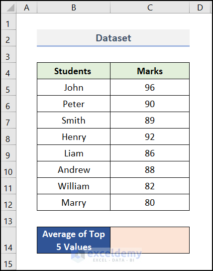
Excel offers us enormous functions. Among them, there are some functions that can be used to an average of the top 5 values in Excel. In addition, we use some other functions to find out the top 5 values and then do the average. Here we make a dataset of Student’s Marks. We want to know the average marks of the top 5 marks.

Not to mention, we have used the Microsoft 365 version. You can use any other version at your convenience.

1. Using AVERAGE and LARGE Functions

Basically, the LARGE function finds out the n-th largest value from the array or range of cells selected based on the serial number. You have to put the number for what the function will find out the largest number. We want to know the top 5 values so we will put the n-th number as 5. The AVERAGE function will then make the average of those values. If you are confused about this method, then follow the steps below to get a proper idea.

📌 Steps:

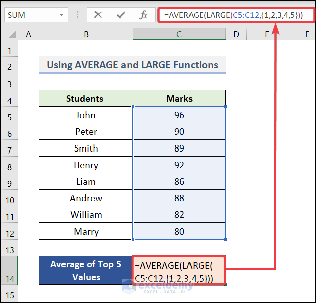
In the very beginning, go to cell C14 where we want to show the average.
Write down the below formula.

=AVERAGE(LARGE(C5:C12,{1,2,3,4,5}))

Here,

C5:C12 = The range of the marks.

Formula Breakdown:

LARGE(C5:C12,{1,2,3,4,5})→ the function finds out the {1,2,3,4,5} (five) largest value among the entire range of C5:C12. Then it returns the top 5 largest values as an output.

Output→ 96,92,90,89,88

AVERAGE(LARGE(C5:C12,{1,2,3,4,5}))→ This function will calculate the average of the returns value of the LARGE function.

Output→ 91

Finally, you will get the average of the top 5 marks.

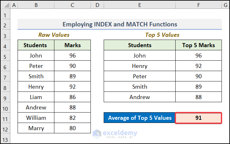
2. Employing INDEX and MATCH Functions

The MATCH function looks out for a specific value among a range of datasets and then returns the position of that value in the cells. Then the INDEX function will return the reference value mentioned by the MATCH function. Here, we will find out the top 5 values with these functions.

📌 Steps:

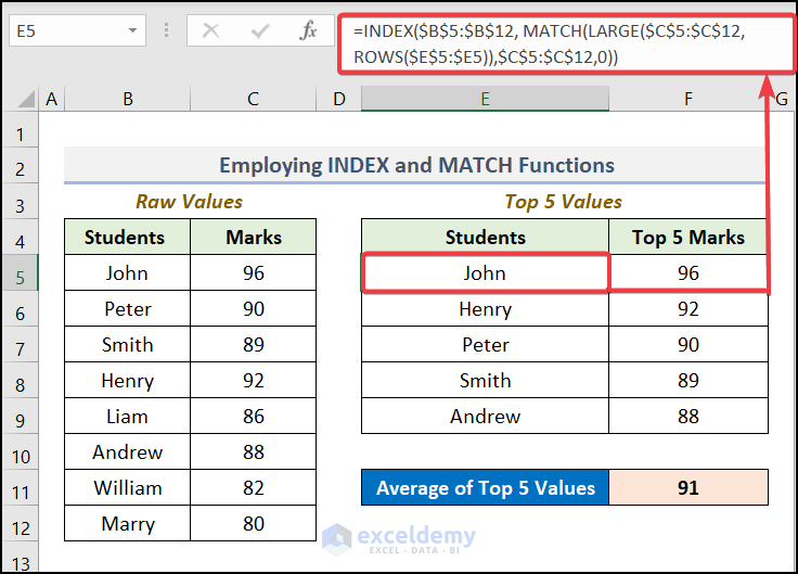
First of all, select cell E5 and write the formula.

=INDEX($B$5:$B$12, MATCH(LARGE($C$5:$C$12,ROWS($E$5:$E6)),$C$5:$C$12,0))

Here,

$B$5:$B$12= refers to the column of the student’s name,
$C$5:$C$12= range of marks,
$E$5:$E6= the cell where we will show the top 5 values.

Formula Breakdown:

ROWS($E$5:$E6)→ ROWS function inputs the serial number for the LARGE function. Here it will take the output of cell E6.
LARGE($C$5:$C$12, ROWS($E$5:$E6)→ The LARGE function finds out the largest value from the array or range of cells selected based on the serial number. It takes the result of the ROWS function and looks for the largest value among cell $C$5:$C$12.
MATCH(LARGE($C$5:$C$12, ROWS($E$5:$E6)),$C$5:$C$12,0)→ MATCH function looks for the obtained largest value in the array of values & returns with the row number of that value.
INDEX($B$5:$B$12, MATCH(LARGE($C$5:$C$12, ROWS($E$5:$E6)),$C$5:$C$12,0))→ INDEX function finally pulls out the name from the Students column of based on that row number found by the MATCH function.

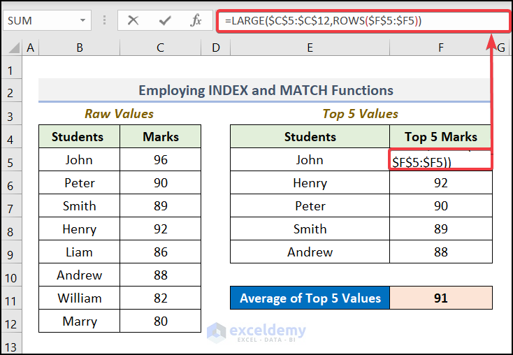
Now, go to cell F5 and write down the formula.

=LARGE($C$5:$C$12,ROWS($F$5:$F5))

LARGE($C$5:$C$12, ROWS($F$5:$F5)) implies that the LARGE function will find out the largest value by taking the serial number produced by the ROWS function.

Later, go to cell F11 and write the formula.

=AVERAGE(F5:F9)

This formula will make an average of the range F5:F9.

Finally, your average of the top 5 values will be displayed.

3. Utilizing XLOOKUP and VLOOKUP Functions

The XLOOKUP function will search from top to bottom of a lookup_array and then return the value corresponding to the first match found by it. Also, we use the LARGE and ROWS functions to get the top 5 values. Then we have done the average of the top 5 values. We demonstrate to you the procedures to use the XLOOKUP function to get the average.

📌 Steps:

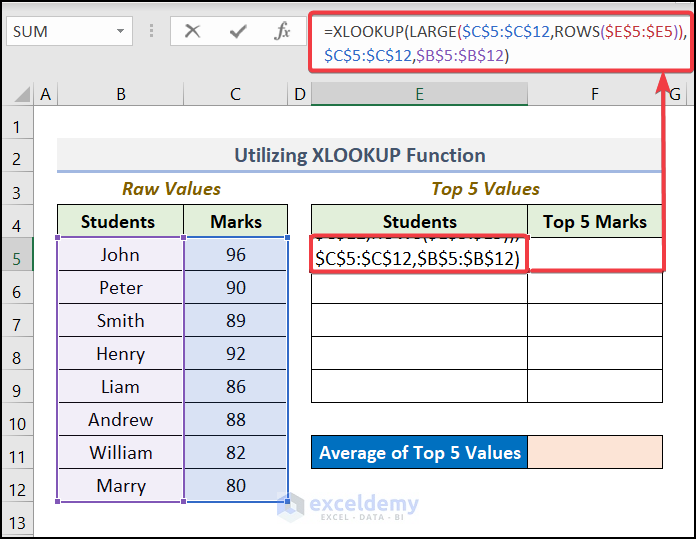
Initially, go to cell E5 and write up the formula.

=XLOOKUP(LARGE($C$5:$C$12,ROWS($E$5:$E5)),$C$5:$C$12,$B$5:$B$12)

Here,

In the 1st argument of the XLOOKUP function, the largest value has been inputted. 2nd argument is the range C5:C12 where the selected largest value will be looked for. The 3rd argument is another range B5:B12 from where the particular data or name will be extracted based on the row number found by the 1st two arguments.

Press ENTER and drag down the Fill Handle tool for other cells.

After that, in cell F5 write down the formula.

=IFERROR(VLOOKUP(E5,B5:C12,2,FALSE),1)

Formula Breakdown:

VLOOKUP(E5, B5:C12,2, FALSE),1)→ VLOOKUP will look for the output for the entered value in cell E5 from the range of B5:C12 and returns the marks for the corresponding value of cell E5.

IFERROR(VLOOKUP(E5, B5:C12,2, FALSE),1)→ This section will find out the error in the argument. If any error occurs, it will return the value.

Afterward, you will get your top 5 values just like the image below.

Lastly, select cell F11 and write up the formula of the average.

=AVERAGE(F5:F9)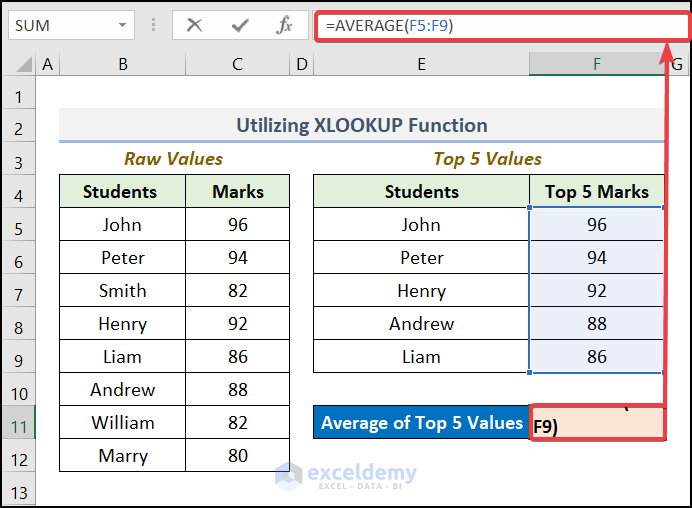

Eventually, your average of the top 5 values will be created.

4. Applying ROW and INDIRECT Functions

Mainly, the ROW function returns the row number of a cell and the INDIRECT function will return a specific reference cell for the given criteria. In this method, we will set a starting number and an ending number then we will apply the formula to get the average of the top 5 values.

📌 Steps:

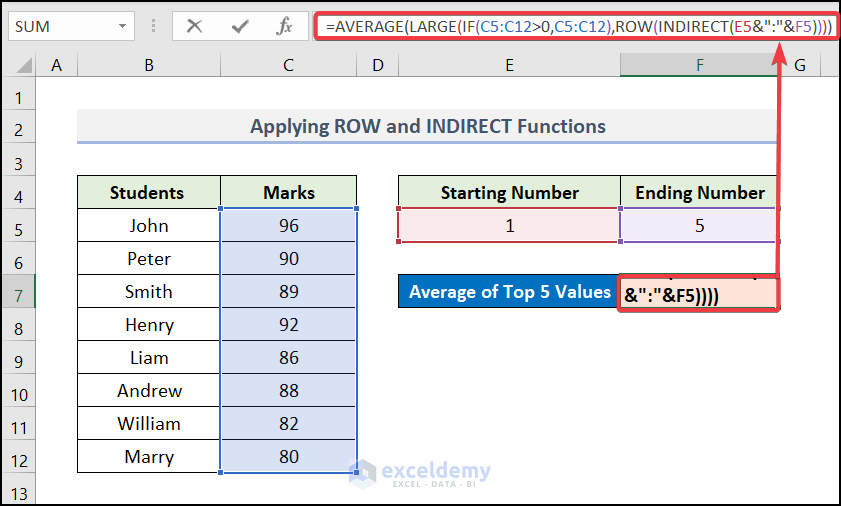
Primarily, go to cell F7 and write the following formula.

=AVERAGE(LARGE(IF(C5:C12>0,C5:C12),ROW(INDIRECT(E5&":"&F5))))

Formula Breakdown:

INDIRECT(E5&”:”&F5)→ This function will lock the reference cells E5 and F5.

ROW(INDIRECT(E5&”:”&F5))→ This function will take the starting number value 1 and ending number value 5.

LARGE(IF(C5:C12>0, C5:C12), ROW(INDIRECT(E5&”:”&F5)))→ The IF function will check if there is any blank cell, if not then the function returns range C5:C12 and as we said before, the LARGE function will find the 5 largest value.

AVERAGE(LARGE(IF(C5:C12>0,C5:C12),ROW(INDIRECT(E5&”:”&F5))))→ This function will calculate the average of the return result.

Finally, you will get result.

5. Using FILTER Function

We will filter the dataset with specific criteria to display the top 5 values among our datasets. Then we will make an average of them. To do this, we use the FILTER function to sort out the value that matches our criteria.

📌 Steps:

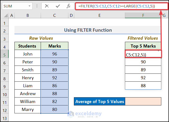
Firstly, move to cell F5 and write down the formula.

=FILTER(C5:C12,C5:C12>=LARGE(C5:C12,5))

Formula Breakdown:

LARGE(C5:C12,5)→ The function will find out the top 5 values as we entered argument 5 among C5:C12.

FILTER(C5:C12, C5:C12>=LARGE(C5:C12,5))→ The FILTER function will filter the range C5:C12 and show the largest 5 values.

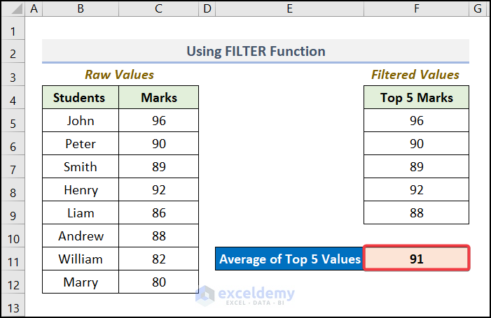
Now, select cell F11 and write the average formula.

=AVERAGE(F5#)

It will calculate the average of the entered argument F5#.

Finally, you will get the result.

Practice Section

We have provided a practice section on each sheet on the right side for your practice. Please do it by yourself.

Download Practice Workbook

Download the following practice workbook. It will help you to realize the topic more clearly.

Average of Top 5 Values.xlsx

Conclusion

That’s all about today’s session. These are some easy methods to an average of the top 5 values in Excel. Please let us know in the comments section if you have any questions or suggestions. For a better understanding please download the practice sheet. Thanks for your patience in reading this article.