Download Practice Workbook
Download the Excel workbook.
Method 1 – Calculating the Simple Arithmetic Average of a Group of Numbers
1.1 Using the Excel AutoSum to Find Average for a Group of Numbers Quickly
This is the sample dataset.
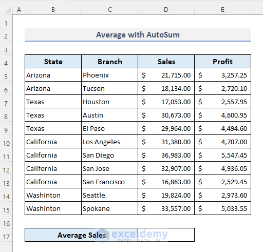
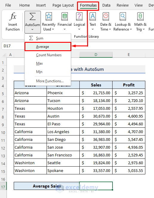
Step 1:
- Select a cell to see the output: D17.
- Go to the Formulas tab.
- In AutoSum, select Average.
Step 2:
- Select the sales values in the Sales column.
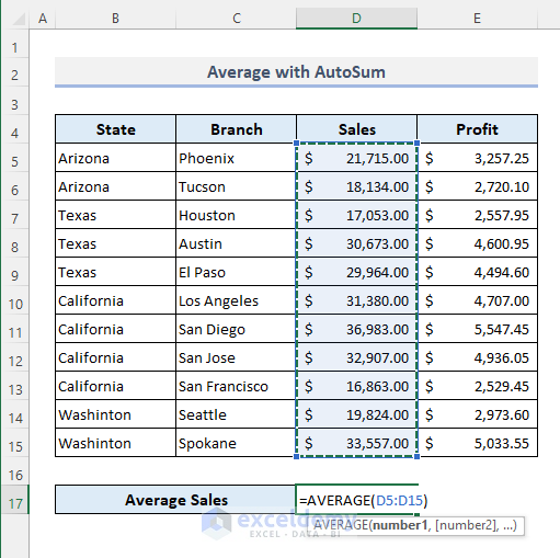
Step 3:
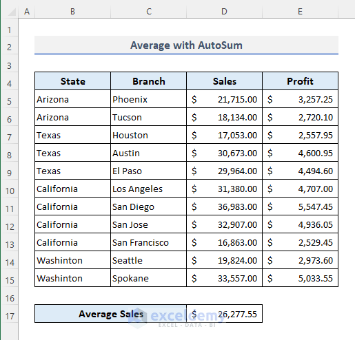
- Press Enter.
You’ll see the average sales in D17.
1.2 Using the Basic AVERAGE Function to Calculate the Average in Excel
- Enter the formula in D17:
=AVERAGE(D5:D15)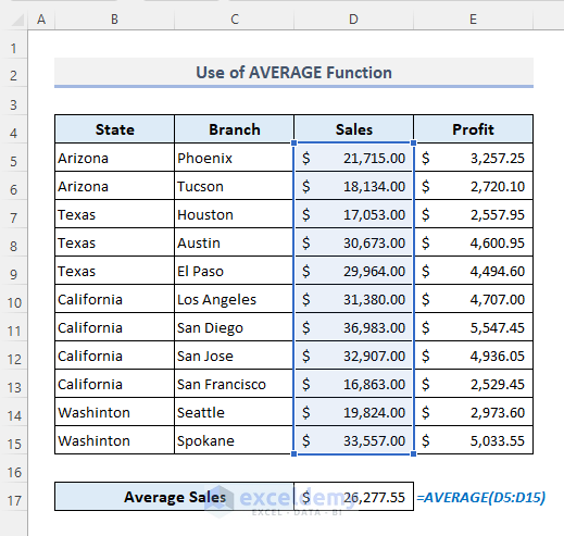
1.3 Finding the Average Manually
Use the formula:
=SUM(D5:D15)/COUNTA(D5:D15)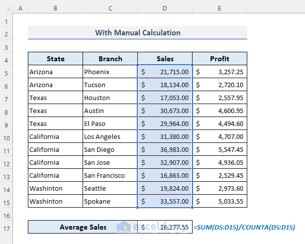
1.4 Using the Excel SUBTOTAL Function to Find the Average
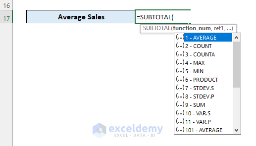
- Enter the formula in D17:
=SUBTOTAL(1,D5:D15)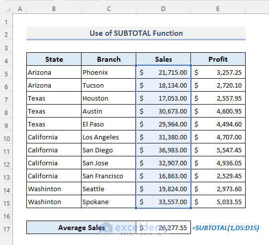
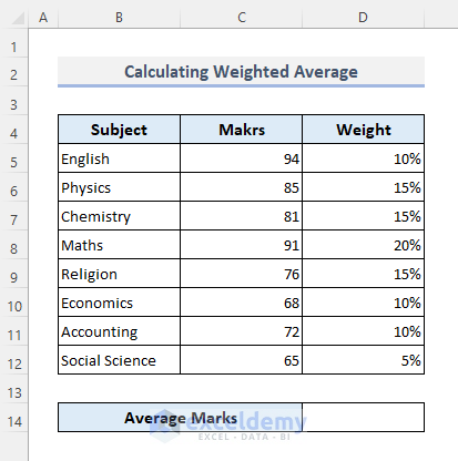
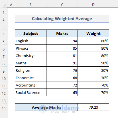
Method 2 – Calculating the Weighted Average with the SUMPRODUCT and the SUM Functions
The dataset below showcases a student’s marks in a final exam. Each subject has a weightage percentage.
To calculate the average marks in D14.
- Use the following formula:
=SUMPRODUCT(C5:C12,D5:D12)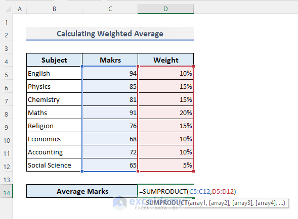
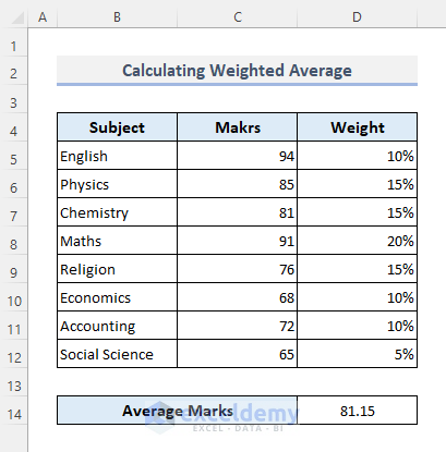
- Press Enter.
This is the output.
If the weightage percentages do not add up to 100%:
- Use the following formula:
=SUMPRODUCT(C5:C12,D5:D12)/SUM(D5:D12)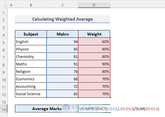
- Press Enter.
This is the output.
Method 3 – Finding the Average with a Single Criterion
To know the average sales of all branches in California:
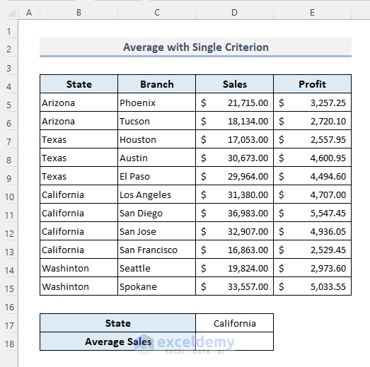
- Select D18.
- Enter the formula:
=AVERAGEIF(B5:B15,D17,D5:D15)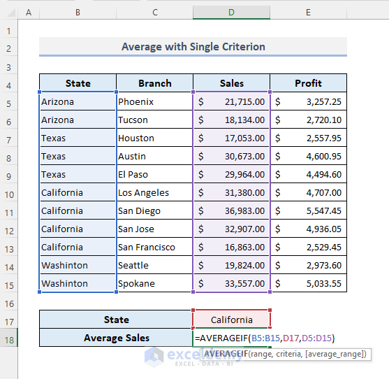
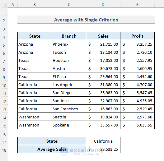
- Press Enter to see the output.
Read More: How to Calculate Average of Multiple Ranges in Excel (3 Methods)
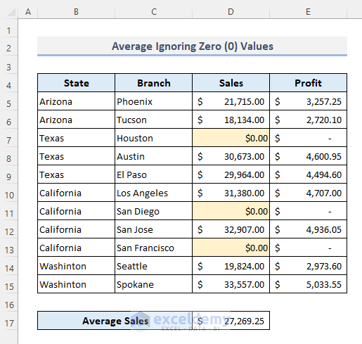
Method 4 – Calculating the Average Ignoring Zero (0) Values
- Select D17.
- Enter the formula:
=AVERAGEIF(D5:D15,"<>"&0)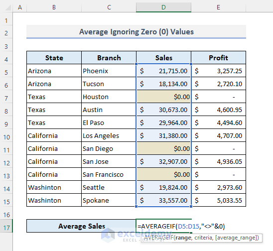
- Press Enter to see the output.
Read More: How to Calculate Average in Excel Excluding 0 (2 Methods)
Method 5 – Calculating the Average with Multiple Criteria in Excel
To know the average sales in California and Texas:
- Enter the formula below:
=AVERAGEIFS(D5:D15,B5:B15,”California”,B5:B15,”Texas”)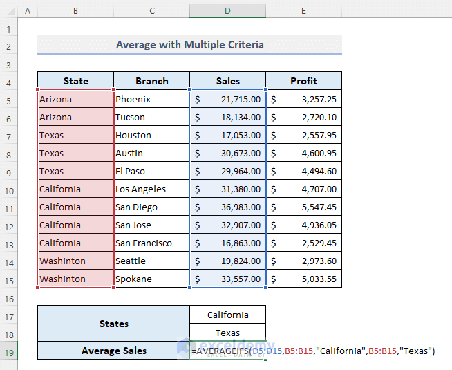
- Press Enter.
The function returns a #DIV/0! error. (It cannot return the output from a single column).
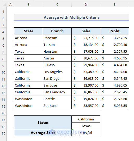
- Use this formula:
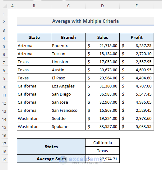
=SUM(SUMIF(B5:B15,D17:D18,D5:D15))/ SUM(COUNTIF(B5:B15,D17:D18))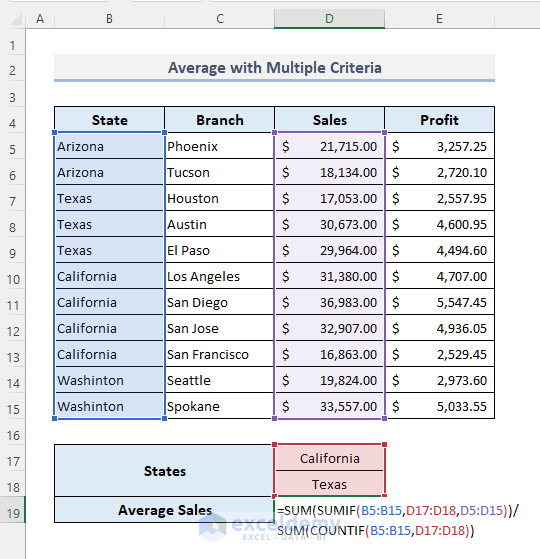
This is the output.
Formula Breakdown
- SUMIF(B5:B15,D17:D18,D5:D15): returns the total sales for California and Texas in an array. The output is: {118133;77690}
- SUM(SUMIF(B5:B15,D17:D18,D5:D15)): adds up the total sales and returns $1,95,823.00.
- COUNTIF(B5:B15,D17:D18): counts cells containing ‘California’ and ‘Texas’ and returns: {4;3}
- SUM(COUNTIF(B5:B15,D17:D18)): sums the total counts and returns 7.
- SUM(SUMIF(B5:B15,D17:D18,D5:D15))/ SUM(COUNTIF(B5:B15,D17:D18)): divides the total sales for California and Texas by the total counts and returns: $27,974.71.
Similar Readings
- How to Calculate Average, Minimum And Maximum in Excel (4 Easy Ways)
- How to Calculate VLOOKUP AVERAGE in Excel (6 Quick Ways)
- Average Attendance Formula in Excel (5 Ways)
- How to Calculate Centered Moving Average in Excel (2 Examples)
Method 6 – Calculating the Average of Top or Bottom 3 with the LARGE or the SMALL Functions in Excel
- Select D17.
- Enter the formula:
=AVERAGE(LARGE(D5:D15,{1,2,3}))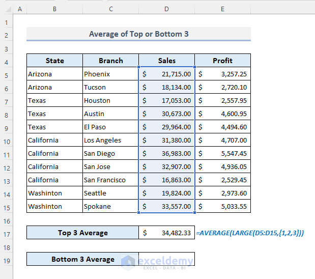
- To determine the average of the bottom 3 sales, use the formula:
=AVERAGE(SMALL(D5:D15,{1,2,3}))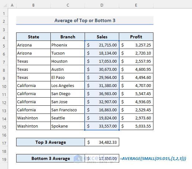
Method 7 –Ignoring the #DIV/0! Error While Calculating the Average in Excel
The #DIV/0! error is displayed when a numeric value is divided by zero (0).
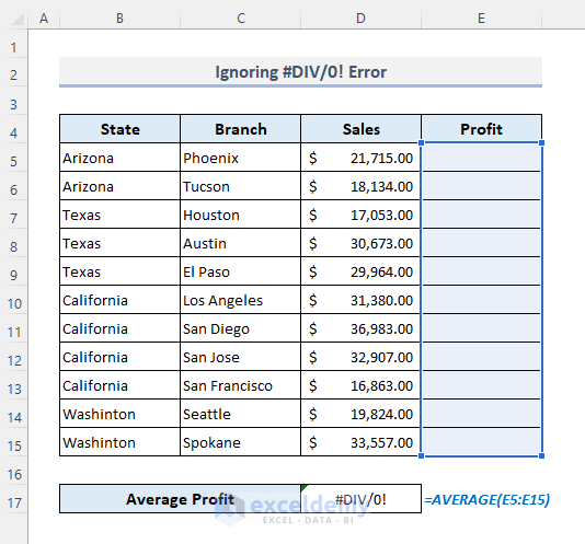
- Select D17.
- Enter the formula:
=IFERROR(AVERAGE(E5:E15),"No Data Found")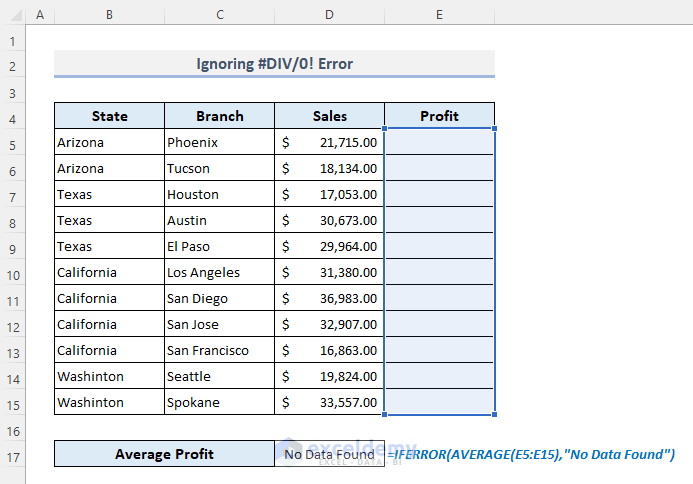
Method 8 – Using the Excel AVERAGEA Function
There are 3 text values in the Sales column.
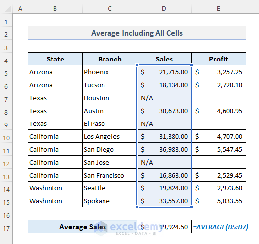
To convert the text values to ‘0’:
- Use the formula:
=AVERAGEA(D5:D15)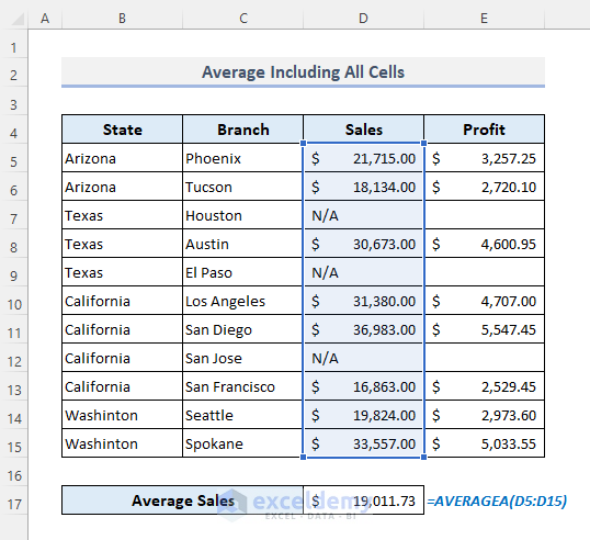
Note: The output must be less than or equal to the output of the AVERAGE function for a similar cell range of cells.
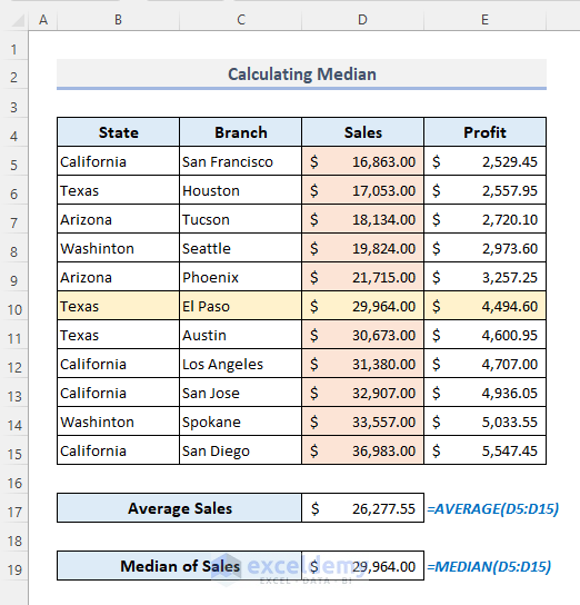
Method 9 – Calculating Other Types of Average in Excel: Median and Mode
9.1 Using the MEDIAN Function
In the dataset below, the average sales value is $26,277.55, but the median is $29,964.00.
- Use the formula:
=MEDIAN(D5:D15)
You can sort the Sales column in ascending or descending order: there are 11 sales values in the column. The median is in the middle or 6th row.
9.2 Using the MODE Function
In the table below, $21,000.00 is displayed thrice in the Sales column.
Use the formula:
=MODE(D5:D15)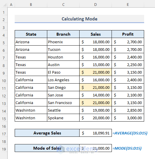
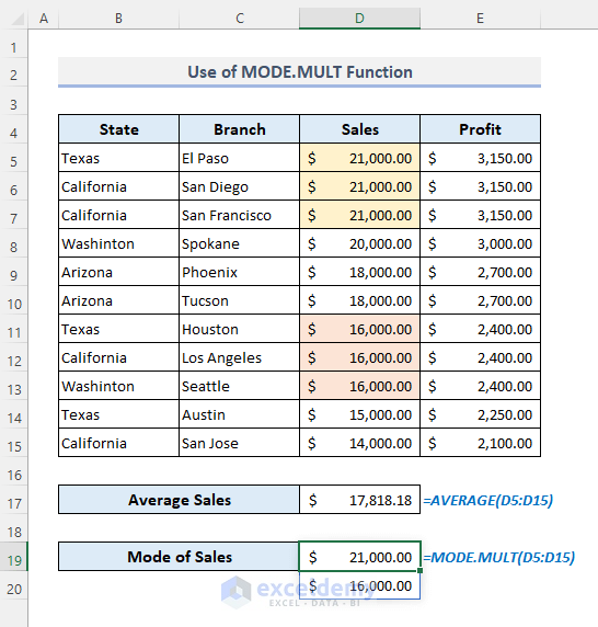
9.3 Using the MODE.MULT Function
In the dataset below, the function returned $16,000.00 although there is a sales value of $21,000.00 with the same number of occurrences as $16,000.00.
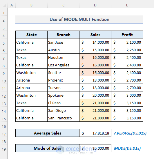
- If you sort the Sales column in descending order, the MODE function will return $21,000.00.
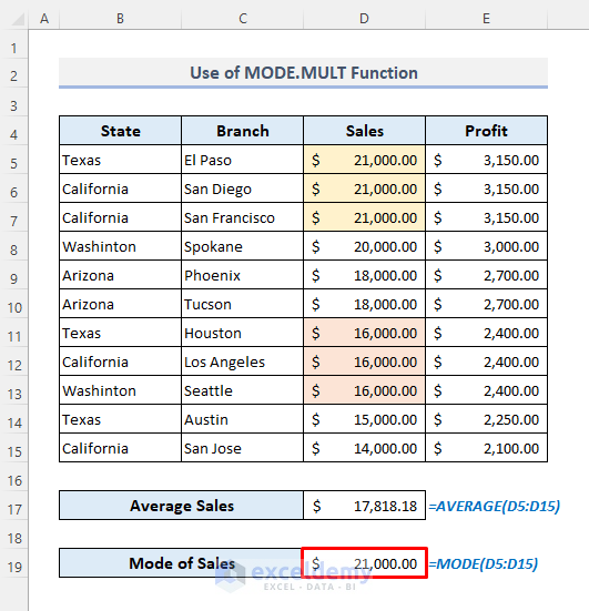
- Use the following formula:
=MODE.MULT(D5:D15)This is the output.
9.4 Using the MODE.SNGL Function
- Use the formula:
=MODE.SNGL(D5:D15)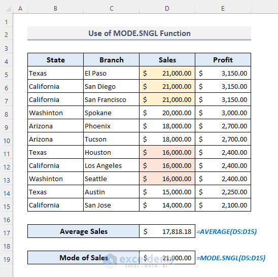
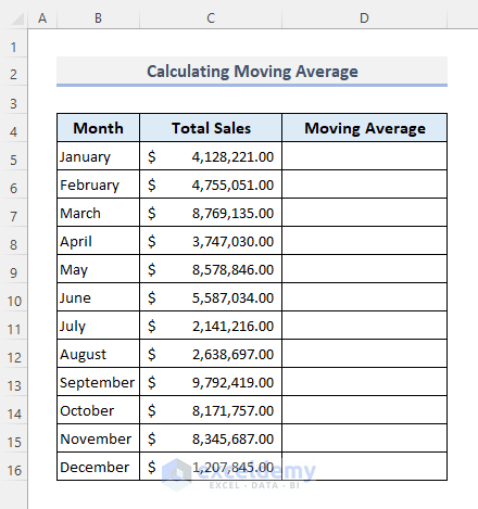
Method 10 – Calculate the Moving Average with the Excel Analysis ToolPak
Calculate the moving average with a specific interval:
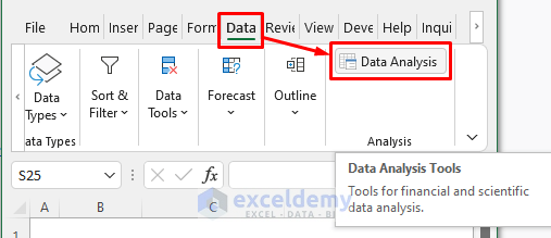
Step 1:
- Go to the Data tab.
- Select Data Analysis in Analysis.
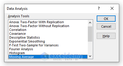
Step 2:
- Choose Moving Average and click OK.
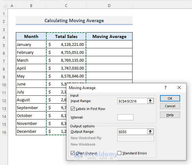
Step 3:
- In Input Range, select the entire column of total sales with its header.
- Check Label in the First Row option.
- Define a cell as the Output Range.
- Check Chart Output.
- Click OK.
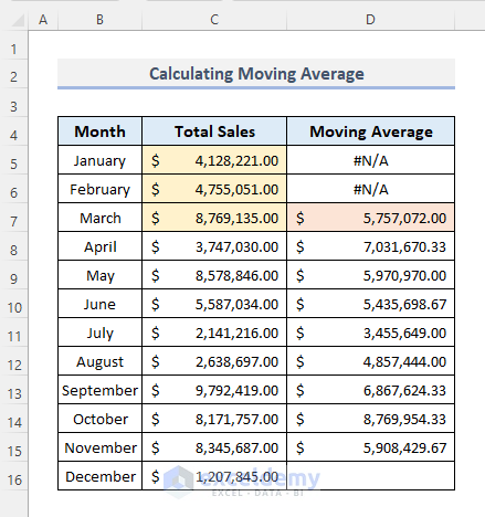
The default interval is 3. The moving average is counted every 3 successive sales values.
This is the output.
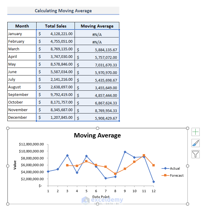
The following chart displays the data points of the total sales and the moving averages. If you click the chart, you will see the reference columns in the data table.
Method 11 – Applying the TRIMMEAN Function to Calculate the Trimmed Mean in Excel
Select the trim percentage as 20% or 0.2.
- Use the formula:
=TRIMMEAN(D5:D15,0.2)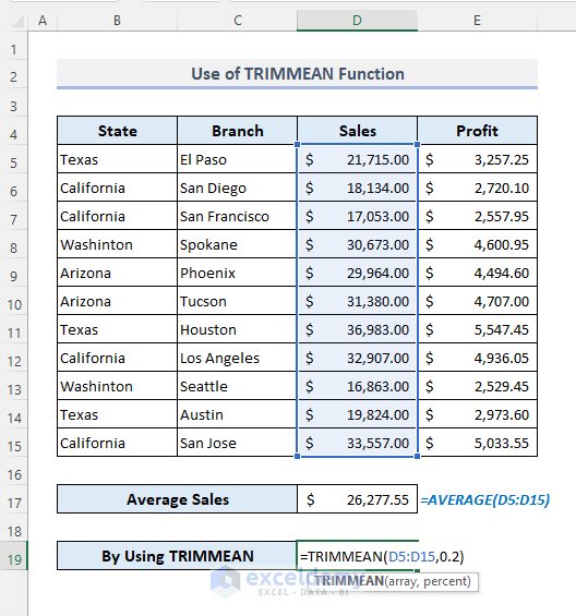
- Press Enter.
You’ll see the average sales of a trimmed sales range.
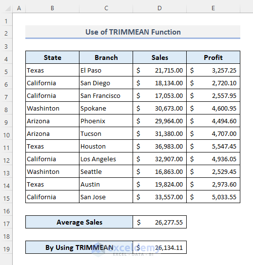
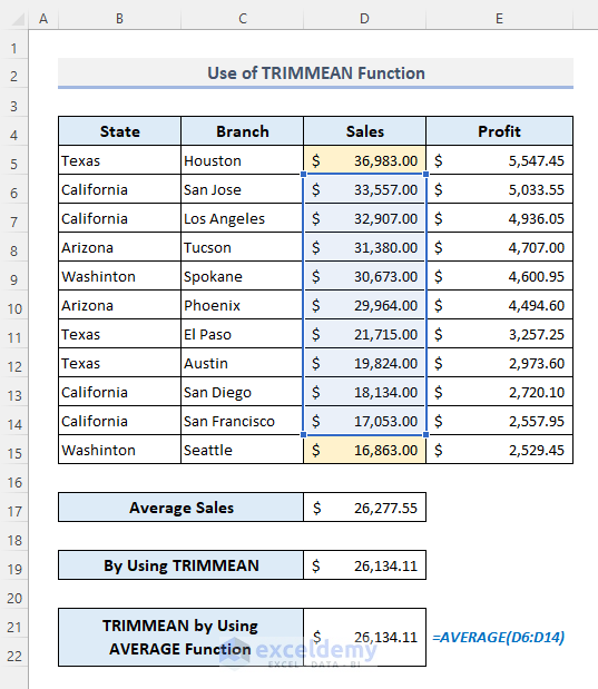
The simple AVERAGE function returns the same value: $26,134.11.
Related Articles
- Running Average: How to Calculate Using Excel’s Average(…) Function
- How to Generate Moving Average in Excel Chart (4 Methods)
- Calculate Moving Average in Excel (4 Examples)
- How to Calculate Exponential Moving Average in Excel
- How to Calculate Percentage above Average in Excel (3 Easy Ways)

