How to Get Sensitivity Report from Solver in Excel

If you have ever used the Excel Solver add-in, you know it is an extremely powerful tool. What you may not know is that Excel Solver can also generate a sensitivity report that can be very helpful in understanding how your solution is affected by changes in the input values. In this article, I will show you how to get a sensitivity report in Excel Solver. So without having any further discussion, let dive straight into it.

What Is a Sensitivity Report?

Sensitivity Reports are a way of analyzing how changes to the inputs of a model affect the outputs of the model. In Excel Solver, a sensitivity report can be generated for a model after the Solve button is clicked.

The sensitivity report lists the values of the objective function and the constraints for the original solution. The report also lists the values of the Shadow Prices, which are the prices that the solver uses to determine how changes in the adjustable cells affect the objective function.

The shadow prices can be used to interpret the results of the sensitivity report. For example, if the shadow price for a constraint is positive, then increasing the value of the adjustable cell associated with that constraint will increase the value of the objective function. If the shadow price for a constraint is negative, then increasing the value of the adjustable cell associated with that constraint will decrease the value of the objective function.

How to Get Sensitivity Report from Solver in Excel

Step-1: Prepare Your Dataset

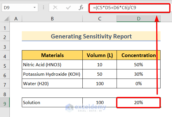
Let’s say we want to make of solution of Nitric Acid, Potassium Hydroxide, and Water. Our target volume of the solution is 100L with 20% concentration.

Currently, we have the following materials:

• Nitric Acid (HNO3): Volume 10L with 50%
• Potassium Hydroxide (KOH): Volume 50L with 30%
• Water (H20): Volume 100L with 0%

We can easily determine our target concentration using the following formula in cell D9.

In this formula,

• C5 is the total volume of Nitric Acid.
• D5 is the concentration of Nitric Acid.
• C6 is the total volume of Potassium Hydroxide.
• D6 is the concentration of Potassium Hydroxide.
• And C9 is the target volume of the final solution.

This formula will return a 20% concentration of the final solution.

Step-2: Set Solver Parameters

Now let’s start generating the sensitivity report. To do that,

❶ Go to the Data tab first.

❷ Then click on the Solver command in the Analysis group.

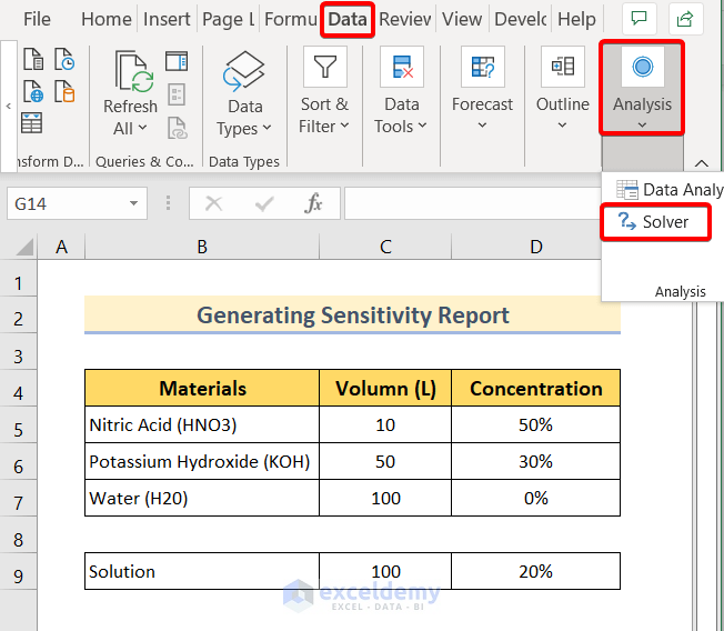
At this point, the Solver Parameters window appears.

❸ In the Set Objective box, insert the cell address of the target concentration of the solution which is cell $D$9.

❹ After that, select the ‘value of’ option and set the value as 0.2 which refers to the final concentration of 20%.

❺ In the ‘By Changing Variable Cells’ box, insert the cell range of the volume of the materials which is $C$5:$C$7.

❻ Then click on the Add button to add constraints in the ‘Subject to the Constraints’ box.

Here I’ve used two constraints which are:

The first constraint means the volume of Nitric Acid can be less than or equal to 10L in the final solution.

The second constraint means the volume of the final solution will be 100L.

After inserting all the solver parameters,

❼ Hit the Solve button.

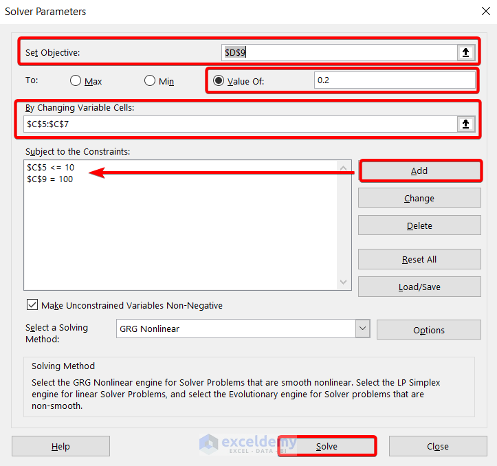
Note: You can choose a solving method from the Select a Solving Method drop-down field, for the example purpose I’ve kept GRG Nonlinear selected, you may need a different method for your scenario.

Read More: How to Do Sensitivity Analysis in Excel

Step-3: Generate Sensitivity Report

To generate a sensitivity report,

❶ Select the ‘Keep Solver Solution’ option in the left column of the Solver Results dialog box.

❷ Then choose Sensitivity in the Reports section.

❸ After that hit the OK button.

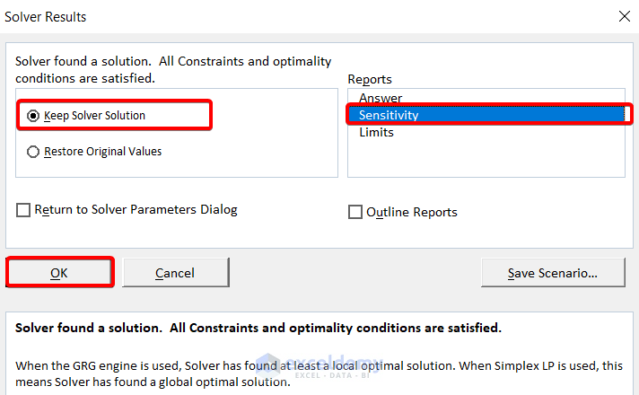
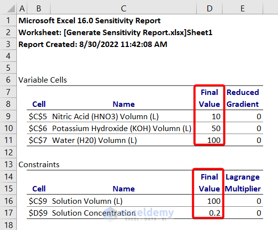
Now the sensitivity report will be automatically generated.

In this report,

You can see the names, corresponding cells, and final values of the variable cells and constraints.

From this report, we can say that 10L Nitric Acid, 50L Potassium Hydroxide, and 100L Water are used to make the final solution of 100L with 20% concentration.

Here the Lagrange Multiplier determines the sensitivity level of the constrained objective to any input changes.

Read More: How to Build a Sensitivity Analysis Table in Excel

Practice Section

You will get an Excel sheet like the following screenshot, at the end of the provided Excel file where you can practice all the topics discussed in this article.

Download Practice Workbook

You can download the Excel file from the following link and practice along with it.

Conclusion

To sum up, I have discussed steps to get a sensitivity report in Excel Solver. Please don’t hesitate to ask any questions in the comment section below. We will try to respond to all the relevant queries asap.

Related Articles

• Sensitivity Analysis for NPV in Excel
• How to Do IRR Sensitivity Analysis in Excel
• How to Perform Sensitivity Analysis for Capital Budgeting in Excel
• How to Use What If Analysis in Excel
• What-If Analysis in Excel with Example
• Types of What-If analysis in Excel
• What If Analysis Data Table Not Working
• How to Delete What If Analysis in Excel

<< Go Back to What-If Analysis in Excel | Learn Excel